Volumes Pre-processing
Volumes Crop
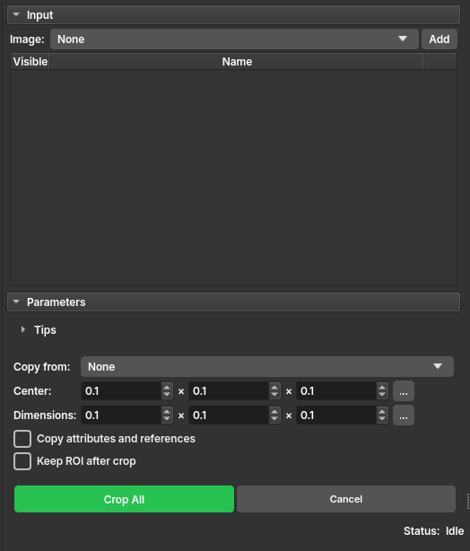
The Volumes Crop module allows for efficient cropping of one or multiple volumes simultaneously using a customizable Region of Interest (ROI). It supports Scalar, Vector, and LabelMap volumes, ensuring that all related data can be processed with a consistent spatial boundary.
Panels and their usage
 |
|---|
| Figure 1: Presentation of the Crop module. |
Main options
Input - Image: Select an image and click Add. You can add multiple images to the list; they will all be cropped using the same ROI configuration. Use the radio buttons in the Visible column to choose which volume to use as a reference in the slice views.
Parameters - Copy from: (Optional) Select an existing ROI to define the crop region. - Center: Set the precise center of the crop in IJK coordinates. Click the ... button to select from the last 10 used configurations. - Dimensions: Define the crop size in the three dimensions (X, Y, Z). Click the ... button to select from the last 10 used configurations. - Copy attributes and references: If checked, the cropped volumes will inherit metadata, attributes, and references from the original volumes. - Keep ROI after crop: If checked, the temporary ROI will be kept as a permanent node in the scene after cropping.
Actions - Crop All/Cancel: Buttons to start the batch cropping process or cancel and clear the list.
Usage
- Select the images to be cropped and add them to the table.
- Adjust the ROI interactively in the slice views or manually via the Center and Dimensions fields.
- (Optional) Hold the Alt key while dragging ROI anchors in the slice views to resize symmetrically around the center.
- Click Crop All and wait for completion. The cropped volumes will appear in the same subject hierarchy folder as the original volumes.
Resample
The Resample module allows changing the spatial resolution of a volume using interpolation, modifying the voxel size along the X, Y, and Z axes. This process is useful for standardizing volumes, by increasing or decreasing their size, or for reducing file sizes for specific analyses that do not require such high resolution.
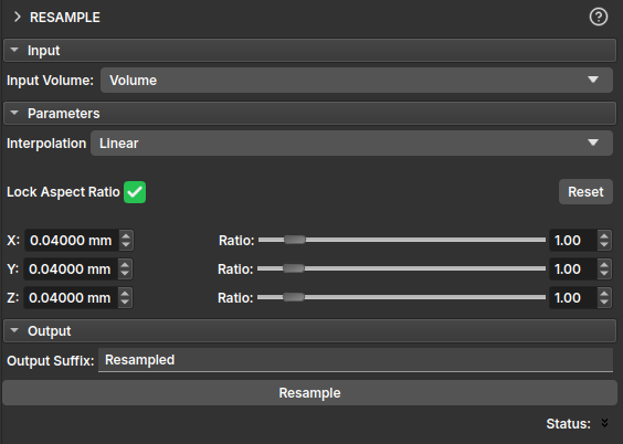
The parameters available in the module are:
- Interpolation: defines the interpolation method used for resampling, which can be:
- Linear: linear interpolation between voxels;
- Nearest Neighbor: assigns the value of the nearest neighbor to the new voxel;
- Lanczos: interpolation based on windowed sinc function. Read more at
;
- Bspline: smooth interpolation using polynomial curves;
- Mean: calculates the average of the original voxels that correspond to the new voxel. Useful for reducing resolution while preserving the general trend of the data.
- Lock Aspect Ratio: when activated, maintains the aspect ratio between the X, Y, and Z axes.
- Reset: restores the original voxel spacing values.
- X / Y / Z: defines the new voxel size in millimeters (mm) for each axis.
- Ratio: shows the change ratio relative to the original voxel size. Can be adjusted manually using the sliders.
- Resample: Executes the resampling process.
Gradient Anisotropic Diffusion
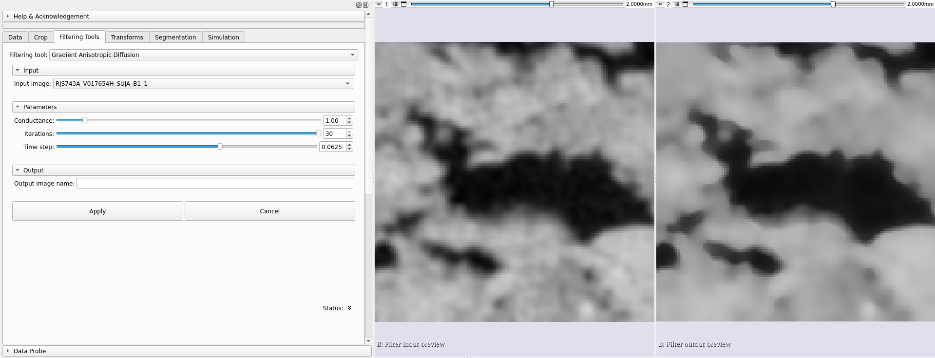
In many applications, it is assumed that transitions from a light to a dark region (characterized by a high gradient) are of interest. While other filters, such as median and Gaussian, often blur boundaries, making pore delimitation more confusing, anisotropic diffusion filters tend to avoid this type of confusion. The conductance term is a function of the image gradient magnitude at each point, reducing the diffusion strength at edges.
 |
|---|
| Left: Original volume, uncorrected. Right: After correction with anisotropic gradient diffusion filter. |
The numerical implementation of this equation available in GeoSlicer is similar to that described in the Perona-Malik paper, but uses a more robust technique for gradient magnitude estimation and is generalized to N-dimensions.
The module parameters for calculating anisotropic gradient diffusion are:
-
Conductance (Conductance): Controls the sensitivity of the conductance term. As a general rule, the lower the value, the more strongly the filter will preserve edges. A high value will cause diffusion (smoothing) of the edges. Note that the number of iterations controls how much smoothing will occur within regions delimited by edges.
-
Iterations (Iterations): More iterations lead to greater smoothing. Each iteration takes the same amount of time. If one iteration takes 10 seconds, 10 iterations take 100 seconds.
-
Time step (Time step): The time step depends on the image dimensionality. For three-dimensional images, the default value of 0.0625 provides a stable solution. In practice, altering this parameter causes few changes to the image.
Curvature Anisotropic Diffusion
Performs anisotropic diffusion on an image using a Modified Curvature Diffusion Equation (MCDE).
MCDE does not exhibit the edge enhancement properties of classic anisotropic diffusion, which under certain conditions can undergo "negative" diffusion, increasing edge contrast. Curvature anisotropic diffusion always undergoes positive diffusion, with the conductance term only varying the strength of this diffusion.
Qualitatively, MCDE compares well with other non-linear diffusion techniques. It is less sensitive to contrast than classic Perona-Malik type diffusion and preserves finer, more detailed structures in images. There is a potential speed disadvantage when using this function instead of the Gradient Anisotropic Diffusion. Each iteration of the solution takes approximately twice as long. Fewer iterations, however, may be necessary to achieve an acceptable solution.
The parameters required for the curvature anisotropic diffusion calculation are the same as those for the anisotropic gradient method.
Gaussian Blur Image Filter
Applies a Gaussian blur filter to the volume; the only parameter is Sigma, representing the width of the Gaussian in mm units.
Median Image Filter
Applies a median filter to the volume; the Neighborhood size parameter defines the neighborhood size in voxels in each of the directions.
Euclidean Distance Transform
Calculates the Euclidean distance transform of a binary image. The output image contains, for each voxel, the distance to the nearest non-zero voxel in the input image.
Usage
- Select the input binary image. Scalar images also work, but only non-zero voxels are considered as foreground.
- If the input has more than one label, select the desired label value to be considered as foreground. It is possible to select multiple segments.
- If the input is a scalar or just have one label, the selection of label value is hidden.
- Choose a prefix for the output image name.
Simple Filters
This module, loaded from the original 3D Slicer, presents a diverse set of filters for calculating binary and grayscale morphology, noise removal, thresholding, image intensity manipulation, region growing, Fourier transform, etc. For a more detailed explanation of each of the options available in this module, consult the specific documentation.
Polynomial Shading Correction
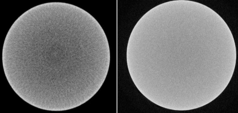
Tomography images often exhibit variations in intensity values that are not characteristic of the sample, but rather of the equipment that collected them. These variations are called artifacts, and there are several types of them. The Polynomial Shading Correction module corrects the artifact known as beam hardening, among others. It is also known as background correction.
 |
|---|
| Left: Beam hardening artifact present. Right: Corrected image after applying shading correction. |
The entire procedure described below is performed slice by slice, in the axial (z-axis) plane of the sample.
For each slice, based on the "Number of fitting points" parameter, a random sample is taken from intensity values at points belonging to the shading mask. These points are used to fit a mathematical function that defines the image background. Depending on the chosen function, this could be a generic Cartesian polynomial, a strict radial polynomial, or a spline profile. For example, a basic second-degree Cartesian polynomial follows this equation:
The fitted function is then used to perform the correction on the slice, following the equation:
Where, \(s'(x,y)\) is the corrected slice, \(s(x,y)\) is the original, and \(M\) is the average of all data in the shading mask (constant value).
The Shading Correction module workflow is divided into three steps: initialization, sampling mask definition, and processing.
Initialization
- Input image: Select the input image you want to correct.
- Keep intermediate image: Check this option if you wish to keep the pre-normalized image generated during the initialization step. This intermediate image facilitates the thresholding step.
- Click the Initialize button. This will pre-normalize the input image and prepare the segment editor for creating the sampling mask.
Threshold
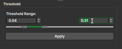
- After initialization, a segment editor interface with the Threshold effect will be displayed to create a mask that covers the image areas affected by shading. This mask will be used to sample points for fitting.
- After adjusting the threshold, click Apply in the Threshold effect panel.
Tip
Consider the mineral in which the beam hardening effect is most clearly appearing. For example: If this is the case for calcite, simply click + drag with the mouse near a region with this mineral; a yellow circle should appear, and you should see the segmentation coloring near the region, depending on the circle's radius.
Tip
For a finer and more sensitive segmentation adjustment, hover your mouse over one of the selection boxes with the maximum/minimum values and use the mouse wheel to increase or decrease the upper/lower limit.
Parameter Selection
- Function: Select the mathematical model used for the shading correction:
- Polynomial: Fits a 2D Cartesian surface. Best for general, non-symmetric shading gradients across the image.
- Polynomial Radial: Fits a curve based strictly on the distance from the center. Best for broad, circular shading effects like standard beam hardening.
- Spline Radial: Calculates a median radial profile and uses splines to handle fine, high-frequency ring artifacts.
- Center: Define the center point for the radial mathematical curve fitting:
- Default: Automatically uses the geometric center of the image (leave "Custom" unchecked).
- Set: Check to manually input the X and Y center coordinates.
- Pick Red View: Click to interactively select the center point directly on the Red slice view.
- Order: Select the complexity of the polynomial curve (2, 4, or 6). Note: This parameter is ignored if 'Spline Radial' is selected.
- Lower orders (2): Capture broad, gentle shading gradients. Less prone to errors.
- Higher orders (6): Allow for more complex, wavy curves but increase the risk of overfitting to local image features instead of the overall shading trend.
- Group size: Define the number of slices that will share the same fitted mathematical function. Smaller values yield better results, but processing is slower as more individual fits must be calculated.
- Fitting points: Define the number of points to be randomly sampled from the mask for the function fitting process. Larger values yield better results, but processing is slower due to the increased computational load of the fitting algorithm.
- Output image name: Enter the desired name for the corrected output image volume.
Apply
- Apply: Click to start the correction process on the input image.
- Apply to full volume: If your input image is a virtual image (lazy node), this button will be visible. Clicking it will open the Polynomial Shading Correction Big Image module, which is optimized for processing large images. The parameters defined in this module will be automatically transferred to the big image module.