Processing
Note
Some features presented on this page will only be available in the private version of GeoSlicer. Learn more by clicking here.
Eccentricity
Ultrasonic image profiles can suffer from eccentricity, which occurs when the tool is not centered in the well. This can cause artifacts in the amplitude image, where one side of the well appears to have systematically lower amplitude than the other. The Eccentricity module corrects these artifacts using transit time to compensate for amplitude variations.
Theory
The correction method is based on patent US2017/0082767, which models amplitude attenuation with distance (related to transit time) using an exponential decay. The key parameter in this model is "Tau".
The correction is applied point by point to the image. The ideal "Tau" value is one that produces a corrected image with certain desired statistical characteristics. The module can optimize "Tau" by minimizing one or more of the following statistical moments of the corrected image's amplitude distribution:
- Standard Deviation: Seeks the smallest amplitude variation in the image.
- Skewness: Seeks an amplitude distribution that is as symmetrical as possible.
- Kurtosis: Seeks an amplitude distribution with "tails" similar to a normal distribution.
How to Use
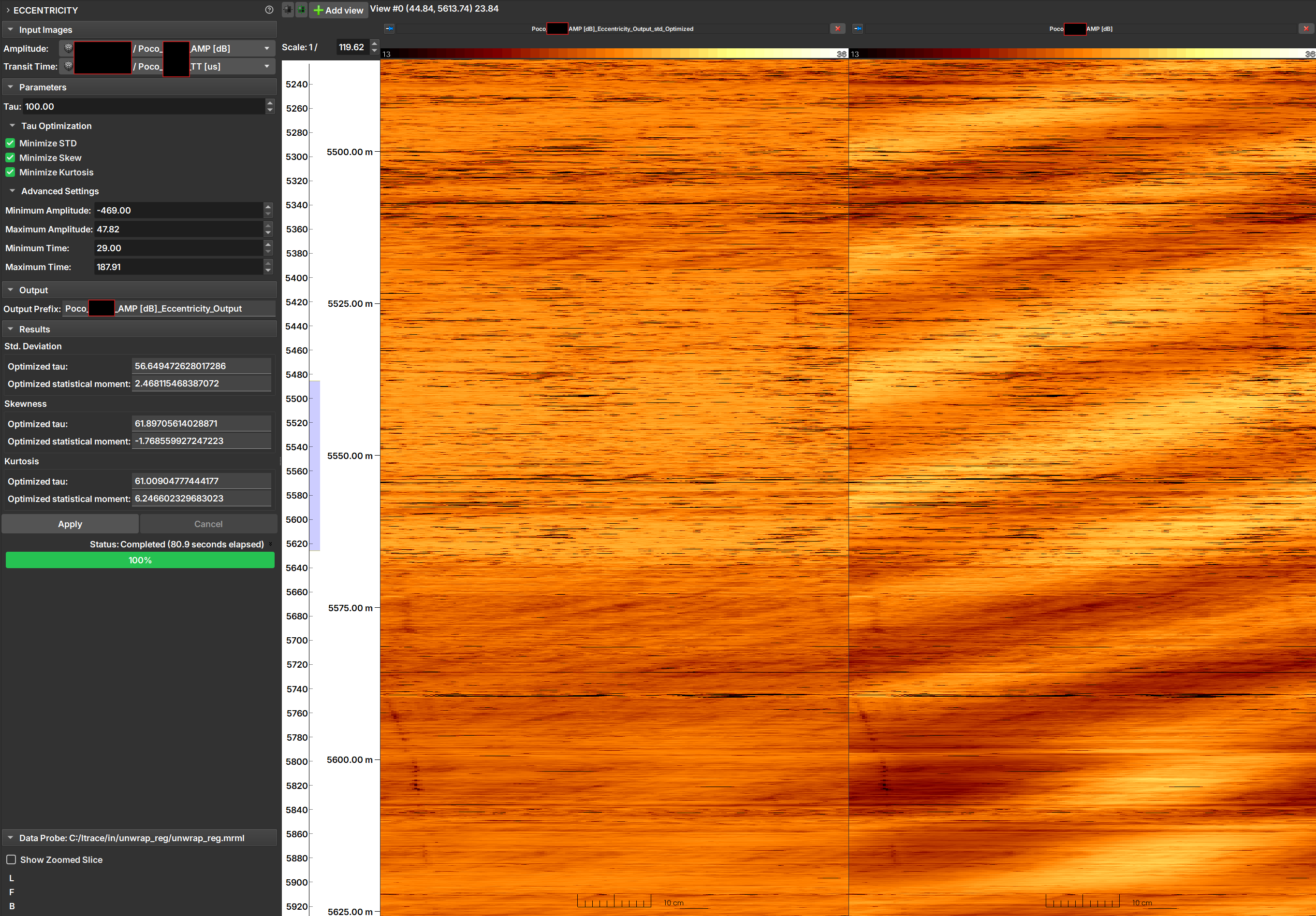 |
|---|
| Figure 1: Eccentricity module interface, result, and original image. |
Input Images
- Amplitude: Select the amplitude image to be corrected.
- Transit Time: Select the corresponding transit time image.
Parameters
- Tau: Enter a "Tau" value to be used for correction. This value is only used if none of the optimization options below are selected.
-
Tau Optimization:
- Minimize STD: Check this option for the module to find the "Tau" that minimizes the standard deviation of the corrected image.
- Minimize Skew: Check to find the "Tau" that minimizes the (absolute) skewness of the corrected image.
- Minimize Kurtosis: Check to find the "Tau" that minimizes the kurtosis of the corrected image.
Note
It is possible to select multiple optimization options. In this case, an output image will be generated for each selected option. If no option is checked, the correction will be performed using the "Tau" value manually entered in the Tau field.
Advanced Settings
This section allows refining the optimization process by ignoring pixel values that might be noise or anomalies.
- Minimum / Maximum Amplitude: Defines the range of amplitude values to be considered in the optimization calculation. Pixels with values outside this range will be ignored.
- Minimum / Maximum Time: Defines the range of transit time values to be considered in the optimization calculation. Pixels with values outside this range will be ignored.
Output
- Output Prefix: Enter the prefix to be used in the name of the output images. The final name will include the optimization type (e.g.,
_std_Optimized).
Results
This section displays the results for each optimization performed.
- Optimized tau: The optimal "Tau" value found by the optimization process.
- Optimized statistical moment: The value of the statistical moment (standard deviation, skewness, or kurtosis) corresponding to the optimized "Tau".
Execution
- Apply: Starts the correction process.
- Cancel: Cancels the execution of the process.
References
- MENEZES, C.; COMPAN, A. L. M.; SURMAS, R. Method to correct eccentricity in ultrasonic image profiles. US Patent No. US2017/0082767. 23 mar. 2017.
Spiral Filter
The Spiral Filter module is a tool designed to remove artifacts from image profiles caused by the spiral movement and eccentricity of the logging tool within the well.
During the acquisition of image profiles, the rotational movement of the tool (spiraling) and its misalignment relative to the center of the well (eccentricity) can introduce periodic noise into the images. This noise appears as a pattern of bands or spirals superimposed on the geological data, which can make the interpretation of true features difficult.
This filter operates in the frequency domain to selectively remove signal components associated with these artifacts, resulting in a cleaner and easier-to-interpret image.
How It Works
The filter is based on applying a band-stop filter to the 2D Fourier transform of the image. The frequency band to be rejected is defined by the vertical wavelengths (in meters) that correspond to the visible spiral pattern in the image. The user can measure these wavelengths directly on the image using the ruler tool to configure the filter parameters.
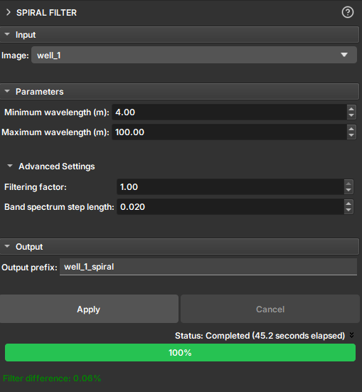
How to Use
- Image: Select the image profile you want to filter.
- Parameters:
- Minimum wavelength (m): Define the minimum vertical wavelength of the spiral artifact. This value corresponds to the smallest vertical repetition distance of the pattern.
- Maximum wavelength (m): Define the maximum vertical wavelength of the artifact.
- Advanced Settings (Optional):
- Filtering factor: Control the filter intensity. A value of
0applies no filtering, while1applies maximum filtering. - Band spectrum step length: Adjusts the smoothness of the filter's frequency band transition. Larger values result in a smoother transition.
- Filtering factor: Control the filter intensity. A value of
- Output prefix: Define the name for the new filtered image volume.
- Click Apply: Press the button to start the filtering process.
Output
The result is a new image volume in the scene with the filter applied. After execution, the Filter difference field displays the percentage of the image that was changed by the filter, providing a quantitative measure of the filtering impact.
Quality Indicator
Well image profiles can be affected by problems during acquisition, such as tool eccentricity (when the tool is not centered in the well) and spiraling (when the tool rotates while moving). These issues introduce artifacts into the data that can hinder interpretation.
The Quality Indicator module calculates an index to quantify the presence and intensity of these artifacts in an image, allowing the user to assess data quality.
Theory
The indicator is calculated based on the 2D Fourier transform of the input image, processed in sliding windows along the depth. The method calculates the average amplitude spectrum within a specific frequency band, which is commonly associated with eccentricity and spiraling effects (vertical wavelengths between 4 and 100 meters and a horizontal wavelength of 360 degrees).
The result is a normalized value between 0 and 1:
- Values close to 0 indicate a low presence of artifacts (high quality).
- Values close to 1 indicate a high presence of artifacts (low quality).
How to Use
Input
- Tempo de Trânsito (Transit Time): Select the input image for the analysis. Although the label suggests "Tempo de Trânsito", any profile image can be used. However, eccentricity and spiraling artifacts are generally more evident in transit time images.
Parameters
- Tamanho da janela (m) (Window size): Defines the size (height) of the sliding window in meters used to calculate the indicator along the well.
- Comprimento de onda mínimo (m) (Minimum wavelength): The minimum vertical wavelength, in meters, to be considered as part of the spiraling effect.
- Comprimento de onda máximo (m) (Maximum wavelength): The maximum vertical wavelength, in meters, to be considered.
Advanced Settings
- Fator de filtragem (Filtering factor): A multiplicative factor for the filter. A value of
0applies no filtering, while1applies maximum filtering. - Passo do espectro da banda (Band spectrum step length): Controls the smoothness of the filter band's roll-off in the frequency domain. Higher values result in a smoother transition.
Output
- Prefixo de saída (Output prefix): Defines the prefix for the name of the generated result.
-
Saída como imagem (Output as image): Controls the format of the result.
- Checked: The result is an image (with the same dimensions as the input) where the value of each pixel is the quality indicator (between 0 and 1).
- Unchecked: The result is a table with two columns:
DEPTH(Profundidade) andQUALITY(Qualidade), which can be viewed as a curve.
Note on Table Output
To optimize performance, the data in the table is a subsampled version (reduced by 10 times) of the full-resolution quality curve. The image output contains the full-resolution data.
Execution
- Apply: Starts the quality indicator calculation.
- Cancel: Stops a process in progress.
Heterogeneity Index
The Heterogeneity Index module (Heterogeneity Index) calculates the heterogeneity index of a well image, as proposed by Oliveira and Gonçalves (2023).
Interface
The module is located in the Well Logs environment. In the left sidebar, navigate through Processing > Heterogeneity Index.
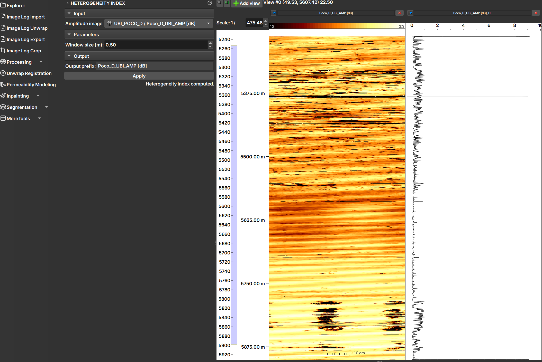 |
|---|
| Figure 1: Heterogeneity Index module (left) and the image visualization next to the index (right). |
Parameters
- Input:
- Amplitude image: Select the amplitude image to be analyzed.
- Parameters:
- Window size (m): Size in meters of the largest depth window to be analyzed. Increasing this value will result in a smoother HI curve.
- Output:
- Output prefix: The output prefix. The output curve will be named as
<prefix>_HI.
- Output prefix: The output prefix. The output curve will be named as
- Apply: Executes the algorithm.
Method
The method calculates the heterogeneity index (HI) of an amplitude image by evaluating the standard deviation at different scales (convolution window sizes). Subsequently, the algorithm fits a linear regression between the logarithm of the scale and the logarithm of the standard deviation. The slope coefficient of this regression represents the heterogeneity index for each analyzed depth. Thus, the index quantifies the relationship between local variation and the observation scale.
References
- OLIVEIRA, Lucas Abreu Blanes de; GONÇALVES, Leonardo. Heterogeneity index from acoustic image logs and its application in core samples representativeness: a case study in the Brazilian pre-salt carbonates. In: SPWLA 64th Annual Logging Symposium, June 10–14, 2023. Proceedings [...]. [S.l.]: Society of Petrophysicists and Well-Log Analysts, 2023. DOI: 10.30632/SPWLA-2023-0034.
Azimuth Shift
The Azimuth Correction module applies a rotation to acoustic image profiles (such as UBI) to correct rotational misalignments caused by tool movement in the well.
Acoustic image profiles are unwrapped in 2D, where one dimension is depth and the other is azimuth (0 to 360 degrees). During acquisition, the logging tool can rotate, which distorts the appearance of geological structures.
This module uses an azimuth table to rotate each image line back to its correct orientation, ensuring that geological features are displayed consistently and interpretably.
How to Use
- Image node: Select the image profile you want to correct.
- Azimuth Table: Choose the table that contains the azimuth data. This table should contain a depth column and a column with the azimuth deviation values in degrees.
- Table Column: Select the specific column in the table that contains the azimuth values to be used for correction.
- Invert Direction (Optional): Check this box if you want the rotation to be applied counter-clockwise. By default, the rotation is clockwise.
- Output prefix: Define the name for the corrected image that will be generated.
- Click Apply: Press the button to start the correction process.
Output
The result is a new image in the project with the azimuthal correction applied.
CLAHE Tool
The CLAHE Tool Module applies Contrast Limit Adaptive Histogram Equalization (CLAHE), "an algorithm for local contrast enhancement, which uses histograms computed over different regions of an image. Thus, local details can be enhanced even in regions lighter or darker than most of the image" - documentation of the equalize_adapthist function from scikit-image on 06/25/2025.
Panels and their usage
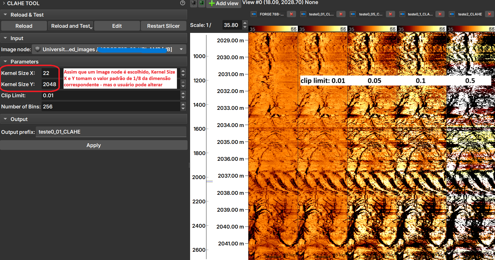 |
|---|
| Figure 1: CLAHE Tool module presentation. |
The image shows the result of applying CLAHE with different clip limit values.
Inputs
- Image Node: Image Log volume to be processed.
Parameters
- Kernel Size: Defines the shape of the contextual regions used in the algorithm. By default, kernel_size is 1/8 of the image height by 1/8 of the width.
- Clip Limit: Normalized between zero 0 and 1. High values result in higher contrast.
- Number of Bins: Number of bins for the histograms ('data range').
Outputs
- Output prefix: Processed image, with float64 type.
KDE of instance measurements
The KDE of instance measurements module allows the calculation of the Kernel Density Estimate (KDE) for a selected property, using the result table generated by the Imagelog Instance Segmenter. The calculation is adjusted according to the depth range and the KDE bandwidth parameter.
Panels and their use
 |
|---|
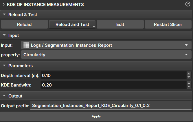
| Figure 1: Presentation of the KDE of instance measurements module. |
Main options
-
Input: Choose Imagelog instance report table.
-
Measurement: Choose Imagelog instance measurement to calculate KDE.
-
Depth interval (m): Choose depth interval to group data.
-
KDE bandwith: KDE bandwidth that controls the smoothness of the estimated density curve.