Big Image
Note
This module is available only in the private version of GeoSlicer. Learn more by clicking here.
The Big Image module is a toolkit for working with large images using limited memory. Visualize slices, crop, downsample resolution, and convert type without loading the entire image into RAM. Currently, it supports loading NetCDF images from multiple local filesystem files or MicroCT NetCDF images from the BIAEP Browser module.
Loading
Follow the steps below to load, preview, and reduce a large image.
Step 1: Load the NetCDF Dataset
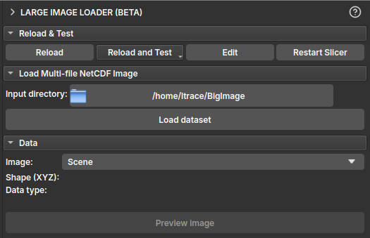
- In the Load Multi-file NetCDF Image section, click the button next to Input directory to select the folder containing the NetCDF file(s) (
.nc). - Once a valid directory is selected, the Load dataset button will be enabled.
- Click Load dataset. This will parse the files' metadata and create virtual images in the GeoSlicer data hierarchy. This operation is fast and does not consume much memory, as the image data is not yet loaded.
Note
A virtual image is an image in the GeoSlicer project that points to the location where a large image is stored. When saving the project, only the image's address is stored in the project folder.
 |
|---|
| Figure 1: "Load Multi-file NetCDF Image" section with the directory selected and the "Load dataset" button enabled. |
Step 2: Select and Inspect the Image
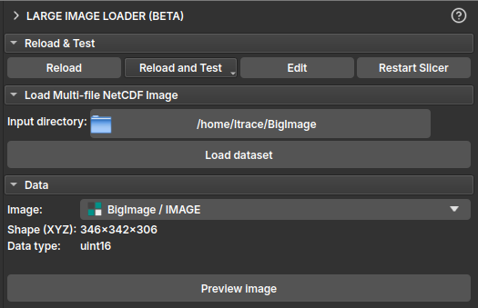
- In the Data section, click the Image selector to view the list of available images in the loaded dataset. Select the image you want to inspect.
- After selection, the Shape (XYZ) and Data type fields will be populated with the information of the selected image.
 |
|---|
| Figure 2: "Data" section showing image selection and populated information fields. |
Step 3: Preview Image Slices
- With an image selected, click the Preview image button to enter preview mode.
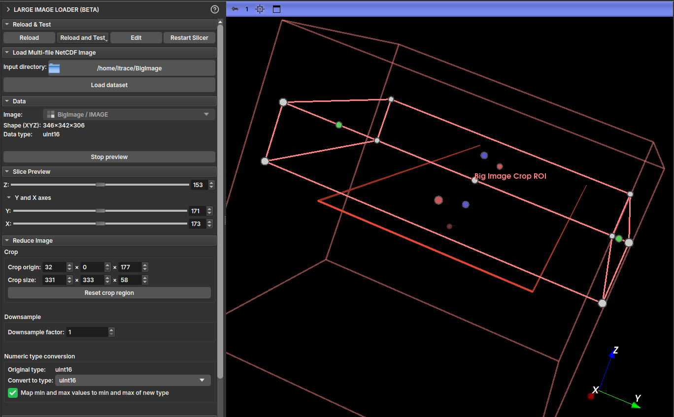
- The Slice Preview section will appear. Use the Z, Y, and X sliders to navigate through image slices in the 2D viewers. Only the selected slice is loaded from disk, allowing exploration of very large images.
- To exit preview mode, click Stop preview.
 |
|---|
| Figure 3: "Slice Preview" section and 2D viewers showing a slice of the large image. |
Note
For NetCDF images saved without chunking, viewing with the Z slider (YX plane) is usually the fastest, while other axes take longer. For images saved with chunking, it is possible to view quickly along any axis.
Tip
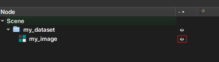
In the Explorer module, you can start previewing an already loaded virtual image by activating its eye icon.
Step 4: Configure Image Reduction
To load a smaller version of the image into memory, configure the options in the Reduce Image section.
- Crop: Define a region of interest (ROI) to crop the image. Specify the starting coordinate in Crop origin and the crop size in Crop size for each axis (X, Y, Z). You can define the crop by interacting with the ROI in the 3D viewer, or by defining the values directly. Use the Reset crop region button to reset the area to the entire image.
- Downsample: Reduce the image resolution by defining a Downsample factor. A factor of 2, for example, will reduce the image size by 8 times (2³).
- Numeric type conversion: Convert the image's numeric type to one that consumes less memory (for example,
uint8).- If the Map min and max values... checkbox is marked, the image values will be remapped to the new type range, preserving the dynamic range.
- If unchecked, values outside the new range will be clamped.
 |
|---|
| Figure 4: "Reduce Image" section with Crop, Downsample, and Type Conversion options highlighted. |
Step 5: Load the Reduced Image
- In the Output section, check the estimated final image size in Output size.
- Define a name for the new volume in Output name.
- Click Load reduced image. The reduction operations (cropping, resampling, and type conversion) will be executed, and the resulting volume will be loaded into GeoSlicer.
 |
|---|
| Figure 5: "Output" section with the output name and "Load reduced image" button highlighted. |
With the reduced image generated, you can visualize it by enabling its display in the Explorer tab.
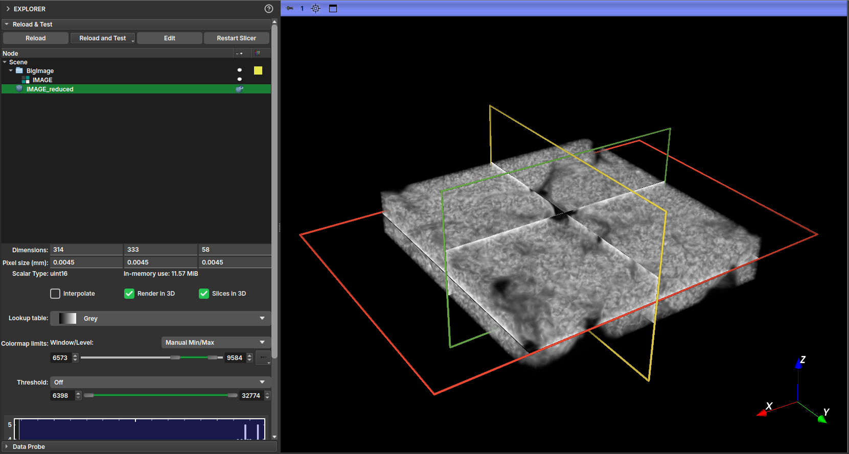 |
|---|
| Figure 6: 3D visualization of the reduced version of the image. |
Polynomial Shading Correction
The Polynomial Shading Correction (Big Image) module is designed to correct shading artifacts or irregular illumination in large-volume images that cannot be entirely loaded into memory. It works by fitting a polynomial to the image background and normalizing the illumination, similar to the Polynomial Shading Correction filter, but with optimizations for out-of-core processing.
This module operates on NetCDF (.nc) files and saves the result to a new file, making it ideal for massive data processing pipelines.
Operating Principle
This module adapts the polynomial shading correction algorithm for images that exceed RAM capacity. The main differences and optimizations are:
- Block Processing (Out-of-Core): The image is divided and processed in blocks (chunks), ensuring that only a portion of the volume is loaded into memory at any given time.
- Point Sampling: To fit the polynomial in each slice, instead of using all pixels from the shading mask, the module randomly selects a defined number of points (
Number of fitting points). This drastically speeds up the fitting calculation without significantly compromising the accuracy of the shading correction. - Slice Grouping: To further optimize the process, the polynomial fit is calculated on the central slice of a group of slices (
Slice group size). The resulting correction function is then applied to all slices within that group.
For a detailed description of the base shading correction algorithm, please refer to the Polynomial Shading Correction filter manual.
Parameters
- Input image: The large-volume image (in NetCDF format) to be corrected.
- Input mask: A mask that defines the region of interest. The area outside this mask will be zeroed in the output image.
- Input shading mask: The mask indicating background areas (or areas with uniform intensity) to be used for point sampling and polynomial fitting.
- Slice group size: Defines the number of slices in a group. The correction is calculated on the central slice and applied to the entire group. A larger value speeds up the process but may not capture rapid shading variations along the slice axis.
- Number of fitting points: The number of points to be randomly sampled from the
Input shading maskto perform the polynomial fitting. - Output Path: The path to the output file in NetCDF (
.nc) format where the corrected image will be saved.
Use Cases
This module is ideal for:
- Preprocessing high-resolution, large-scale micro-computed tomographies (µCT).
- Correcting illumination in image mosaics or any voluminous image that does not fit in memory.
- Normalizing illumination gradients in large datasets before segmentation or quantitative analysis.
Boundary Removal
This module removes the boundaries of a segmentation in a large image (NetCDF format). For more information about the interactive version of this tool, see the Boundary Removal effect in the Segment Editor.
Panels and their use
Input
- Input Image: Select the input image in NetCDF format.
- Segmentation: Select the segmentation node related to the dataset.
Parameters
- Threshold adjustment: Define the threshold range for boundary detection.
Output
- Output Path: Select the output path for the resulting image in .nc format.
Apply Button
- Apply: Initiates the boundary removal process.
Expand Segments
This module expands the segments in a segmentation to fill the entire volume of a large image (NetCDF format). For more information on the interactive version of this tool, see the Expand Segments effect in the Segment Editor.
Panels and their use
Input
- Segmentation: Select the segmentation node related to the dataset.
Output
- Output Path: Select the output path for the resulting image in .nc format.
Apply Button
- Apply: Starts the segment expansion process.
Multiple Threshold
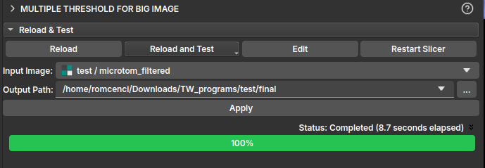
This module is used to segment a sample loaded via Big Image mode from a manual segmentation by Multiple Threshold.
To use this feature, first load the reduced image from the Large Image Loader module. Once loaded, navigate to the module in Manual Segmentation and click the Multiple threshold icon. After selecting the thresholds and performing the segmentation on the reduced image, click Apply to full volume. This should redirect to the current module's page, where the output path to save the result will be chosen.
Virtual Segmentation Flow
Flow for obtaining a porosity map from a scalar volume.
%%{
  init: {
    'themeVariables': {
      'lineColor': '#c4c4c4'
    }
  }
}%%
flowchart LR
    Start --> Import
    Import --> Segmentation
    Segmentation --> Modelling
    Modelling --> Results

    click Segmentation "../../Segmentation/segmentation.html" "teste de imagem"
    style Start fill:#808080,stroke:#333,stroke-width:1px,color:#fff;
    style Import fill:#6d8873,stroke:#333,stroke-width:1px,color:#fff;
    style Segmentation fill:#5a9b87,stroke:#333,stroke-width:1px,color:#fff;
    style Modelling fill:#45ae97,stroke:#333,stroke-width:1px,color:#fff;
    style Results fill:#2ea67e,stroke:#333,stroke-width:1px,color:#fff;

    Segmentation["Segmentation"]
graph LR
    hello --> world
    world --> again
    again --> hello
-
Start Geoslicer in the Volumes environment from the application interface.
-
Select the input volume by clicking on "Escolher pasta" or "Escolher arquivo" and choose the desired import data from the available options. We suggest testing the default parameters first.
-
Select the input volume by clicking on "Input:" Adjust the parameters for different segmentation effects, such as "Múltiplos Limiares," "Remoção de Fronteira," and "Expandir Segmentos." Adjust the settings to achieve the desired segmentation results, using interface feedback and visualization tools.
-
Review and refine the segmented data. Adjust segmentation boundaries, merge or split segments, and apply other modifications to enhance the porosity model using the provided tools.
-
Save the porosity map or export the volume with the parameter tables.
%%{init: { 'logLevel': 'debug', 'theme': 'default','themeVariables': {
            'git0': '#808080',
            'git1': '#6d8873',
            'git2': '#5a9b87',
            'git3': '#45ae97',
            'git4': '#2ea67e',
            'git5': '#ffff00',
            'git6': '#ff00ff',
            'git7': '#00ffff',
            'gitBranchLabel0': '#ffffff',
            'gitBranchLabel1': '#ffffff',
            'gitBranchLabel2': '#ffffff',
            'gitBranchLabel3': '#ffffff',
            'gitBranchLabel4': '#ffffff',
            'gitBranchLabel5': '#ffffff',
            'gitBranchLabel6': '#ffffff',
            'gitBranchLabel7': '#ffffff',
            'gitBranchLabel8': '#ffffff',
            'gitBranchLabel9': '#ffffff',
            'commitLabelColor': '#afafaf',
              'commitLabelBackground': '#0000',
              'commitLabelFontSize': '13px'
       }, 'gitGraph': {'showBranches': true, 'showCommitLabel':true,'mainBranchName': 'Start'}} }%%
      gitGraph LR:
        commit id:"Start"
        commit id:"Volumes  ."
        branch "Import"
        commit id:"Data Tab"
        commit id:"Import Tab"
        commit id:"Select file"
        commit id:"Parameters"
        commit id:"Load  ."
        branch "Segmentation"
        commit id:"Segmentation Tab"
        commit id:"Add new segmentation node"
        commit id:"Create at least 4 segments"
        commit id:"Add ROI  ."
        branch Modelling
        commit id:"Modelling Tab"
        commit id:"Segmentation"
        commit id:"Select Volume"
        commit id:"Select Segmentation"
        commit id:"Apply  ."
        branch Results
        commit id:"Charts"
        commit id:"Images"
        commit id:"Tables"
        commit id:"Reportsd"
Start
Start Geoslicer in the MicroCT environment from the application interface.
Import(TODO)
Select the input volume by clicking on "Escolher pasta" or "Escolher arquivo" and choose the desired import data from the available options. We suggest testing the default parameters first.
Segmentation
Select the input volume by clicking on "Input:" Adjust the parameters for different segmentation effects, such as:
- Multiple Thresholds(TODO)
- Boundary Removal(TODO)
- Expand Segments(TODO)
Adjust the settings to obtain the desired segmentation results, using interface feedback and visualization tools.
Modeling(TODO)
Review and refine the segmented data. Adjust segmentation boundaries, merge or split segments, and apply other modifications to enhance the segmentation model using the provided tools.(TODO)
Results(TODO)
Save the project or export the segmented volume. The results can be displayed as:
- Image(Screenshot)(TODO)
- Graphs(Charts)(TODO)
- Served via Reports (Streamlit)(TODO)