Flows

Geolog Integration

The Geolog Integration Module was developed to establish an efficient connection with the Geolog software, facilitating the import and export of image log data between the softwares. For its full operation, it is necessary to use Python 3.8 in Geolog, as this version includes essential libraries for the integration.

Panels and their usage

Reading a Geolog project

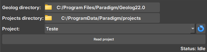
Widget responsible for checking if Geolog is available and reading a Geolog project, checking available WELLS, SETS, and LOGS.


Figure 1: Geolog connection widget.

Geolog directory: Geolog installation directory.
Projects directory: Directory of the folder with the project to be read.
Project: Selector for available projects within the directory. If necessary, the button next to it updates the selector to show new projects.

Importing data from Geolog

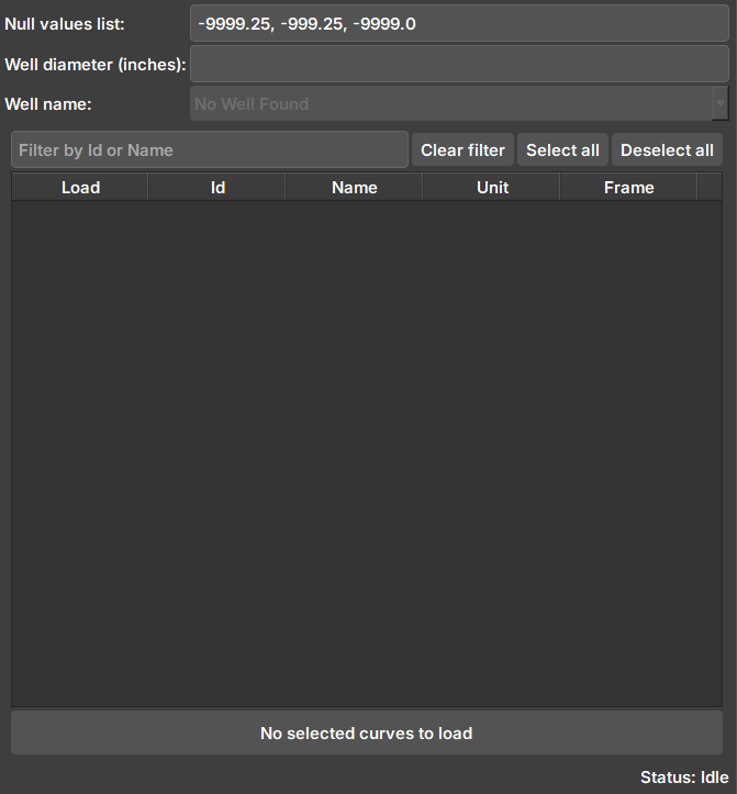
Widget responsible for showing available data for import from Geolog to Geoslicer.


Figure 2: Geolog data import widget.

Null values list: Values considered as null. Imported images are checked if they contain the values in the list and undergo processing.
Well diameter: Well diameter (inches). Used in the calculation of pixels and attributes of the created volume.
Well name: Well name in Geolog. Contains the SETS and LOGS to be imported.
Selector: After connecting and selecting a well, the available data (LOGS) to be imported will appear here.

Exporting data to Geolog

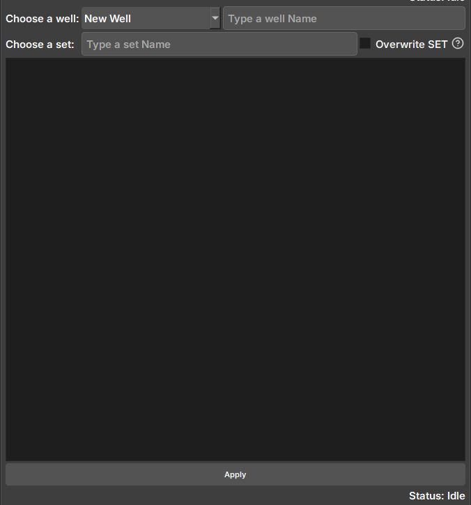
Widget responsible for selecting and exporting image log data from Geoslicer to Geolog.


Figure 3: Geolog data export widget.

Choose a well: Selector for available Wells in the project. Selecting the "New Well" option will create a new well during export, with the name entered in the adjacent field.
Choose a set: Field to enter the name of the SET where the data will be saved. SETs cannot be modified, and choosing an existing SET may overwrite the data if the option next to it is selected.
Selector: Selector for Geoslicer data to be exported. Due to the way writing occurs in Geolog, volumes must have the same vertical pixel size to avoid data failures.

Video: Importing and exporting to Geolog

Image Log Crop

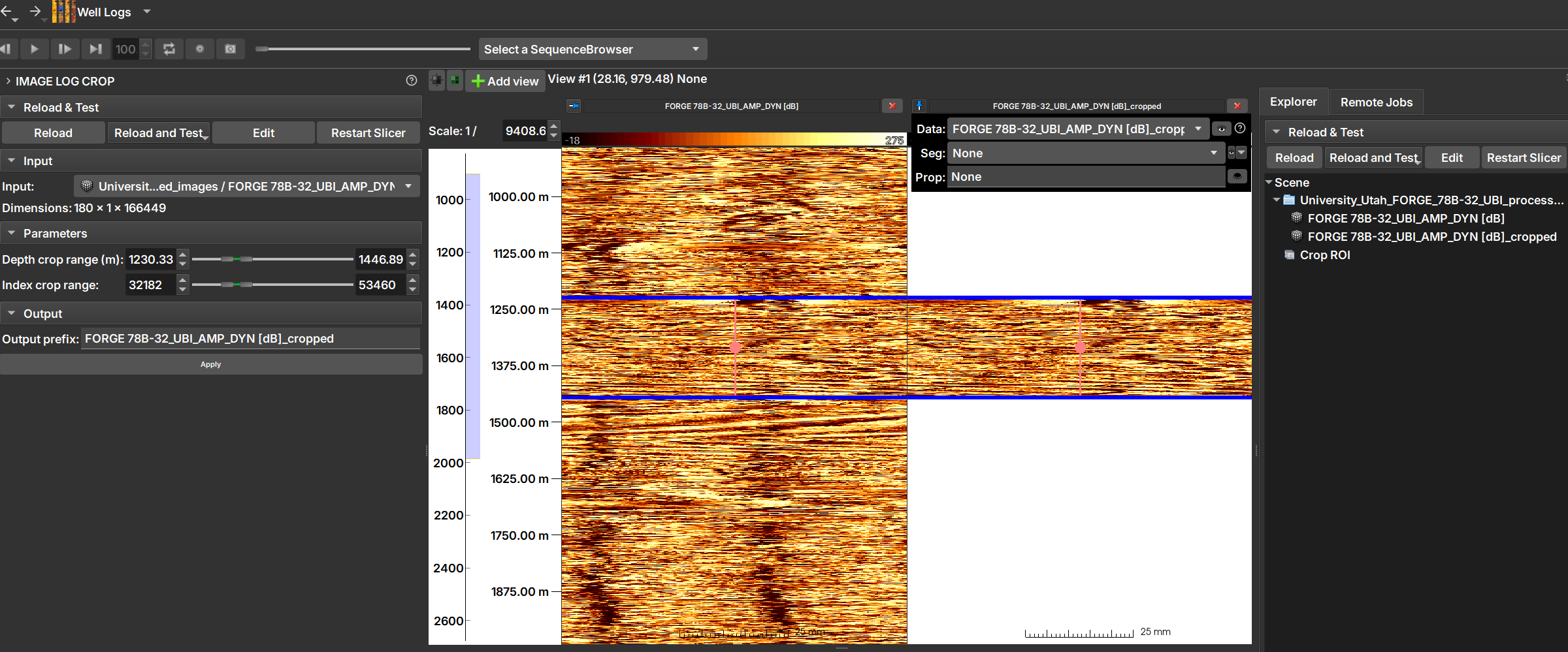
The Image Log Crop Module allows custom cropping of well images, adjusted based on the top and bottom depths of the image.

Panels and their use


Figure 1: Manipulation can be done using sliders and numerical values (on the left), or by dragging the crop region with the mouse over the well image (in the center). After clicking "Apply", the cropped image can be opened and viewed, as shown in the image on the right.

Sliders manipulations (on the left in Image 1) are automatically reflected in the crop region (in the center of the image) and vice-versa.

Main options

Input: Choose the image to be cropped.
Depth crop range (m): Lower and upper limits of the depth range that will constitute the crop, in meters.
Index crop range: The same limits as above, but expressed in indices.
By dragging the crop region with the mouse over the well image (in the center)

Video: Cortando uma imagem de poço

Image Log Inpaint

The Image Log Inpaint Module integrated into GeoSlicer is an inpainting tool that allows interactive inpainting of missing or damaged areas in well images, with dynamic adjustments during the process.

Panels and their usage


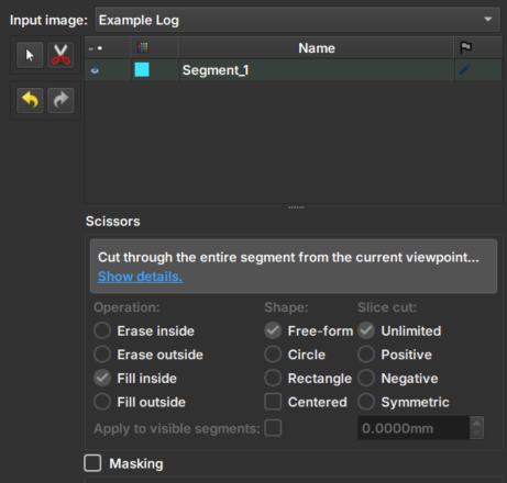
Figure 1: Presentation of the Image Log Crop module.

Main options

Input image: Choose the image to be inpainted. When an image is chosen, two views will be automatically added to facilitate usability.
Clone Volume: Creates a new image to be used in the module, keeping the original image unchanged.
Rename Volume: Renames the chosen image.
Tesoura/Scissors: Tool that performs the inpainting: first, select the tool and then draw on the image the area where the inpainting should be performed. The tool options in the bottom menu are disabled in this module.
Arrows: Allow to undo or redo an inpainting modification.

Video: Filling in the empty spaces of a well image

## Image Generation

The Multiscale Image Generation module offers an interface with various parameters for manipulating and configuring the MPSlib library. MPSlib features a set of algorithms based on multiple point statistical (MPS) models inferred from a training image.
Currently, only the Generalized ENESIM algorithm with direct sampling (DS) mode is available.

### Panels and their use

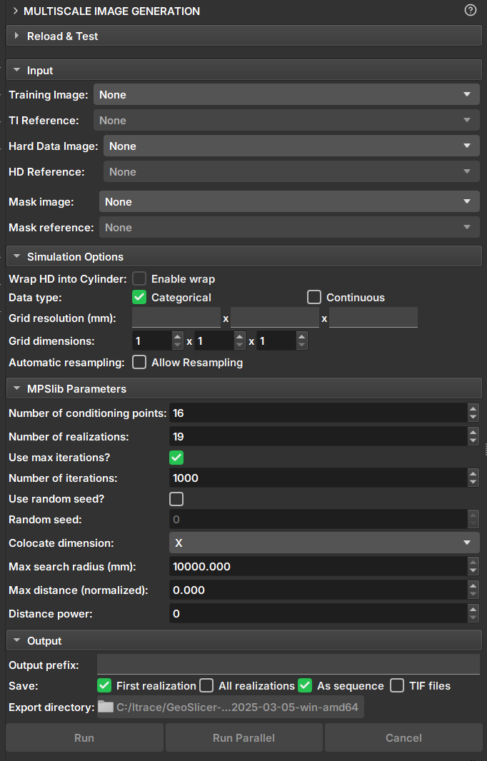
| ![Figure 1](../../assets/images/Multiscale.png) |
|:-----------------------------------------------:|
| Figure 1: Multiscale Image Generation Module. |

#### Input Data

 - _Training Image_: Volume that acts as a training image.

 - _Hard Data Image_: Volume that acts as "Hard Data", where values and points are fixed during the simulation.

 - _Mask Image_: Volume that acts as a mask for selecting the simulation area. Unselected segments will not be included in the simulation.

#### Simulation Options

 - _Wrap HD into cylinder_: If the "Hard Data" is a well image (2D), this option causes the image to be considered a cylinder and performs simulations as 3D.

 - _Data type_: Determines whether the data type is continuous or categorical. Segmentations and Labelmaps can be used for discrete and continuous simulations, but scalar volumes can only be used for continuous.
   - Categorical: Segmentations control regions and determine the class value of the Hard Data and Training Image volume. Unselected segments will be disregarded.
   - Continuous: Segmentations control which regions and volume values will be used as Hard Data or training data. Unselected segments will be disregarded.

 - _Grid Resolution_: Voxel resolution of the resulting image (mm).

 - _Grid Dimensions_: Dimensions of the resulting image.

 - _Automatic resampling_: Activates the automatic resizing functionality of the input data to the simulation grid's dimension and resolution. If the image is an imagelog, Y-axis resizing is disabled.
    - _Spacing_: New axis resolution after resizing.
    - _Size_: New axis dimension after resizing.
    - _Ratio_: Ratio of the new voxel resolution to the initial resolution.

#### Parameters

 - _Number of Conditioning points_: Number of conditioning points to be used in each iteration.

 - _Number of realizations_: Number of simulations and images to be generated.

 - _Number of iterations_: Maximum number of iterations when searching the training image.

 - _Random seed_: Initial value used to start the simulation. The same seed with the same parameters always generates the same result.

 - _Colocate dimensions_: For a 3D simulation, ensure that the order in the last dimensions is important, allowing a 2D co-simulation with conditional data in the third dimension.

 - _Max search radius_: Only conditional data within a defined radius is used as conditioning data.

 - _Max distance (normalized)_: The maximum distance that will lead to the acceptance of a conditional model match. If the value is 0, a perfect match will be sought.

 - _Distance power_: Weights the conditioning data based on the distance from the central values. A value of 0 configures no weighting. 

#### Output Options

 - _Output prefix_: Name of the generated volume or file. In case of multiple realizations, a number is added to indicate the realization.

 - _Save_: Options for saving the results.
   - _First realization_: Saves only the first realization as an individual volume.
   - _All realizations_: Saves all realizations as individual volumes.
   - _As sequence_: Saves the realizations in a sequence set. The "_proxy" output volume indicates it is a sequence and has the controllers for visualizing the realizations.
   - _TIF files_: Saves all realizations as tiff files.

 - _Export directory_: Directory where the tiff files will be saved. It is only enabled if the "TIF files" option is selected.

#### Buttons

- _Run_: Executes the mps sequentially. The _Geoslicer_ interface is locked during the execution of this option.
- _Run Parallel_: Executes the mps in parallel. In this option, the execution runs in another thread, and the interface can be used during execution.
- _Cancel_: Interrupts the simulation execution. Only when executed in parallel.


<figure class="video-container">  <video controls width="100%">  <source src="../../../assets/videos/multiscale_multiscale.webm" type="video/webm" >  Your browser does not support the video tag.</video>  <figcaption>Video: Simulando um volume 3D a partir de uma imagem de poço</figcaption></figure>

Post Processing

Module for data extraction after Multiscale simulation.


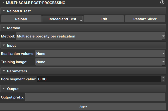
Figure 1: Multiscale Post Processing Module.

Methods

Porosity per Realization

Produces a table with the porosity percentage of each slice of a volume, across all volumes in a sequence.

Input Data and Parameters

Result Volume: Volume for porosity calculation. If the volume is a proxy for a sequence of volumes, porosity will be calculated for all realizations.
Training Image: Extra volume included in the calculations and added to the table as a reference.
Pore segment Value: Value to be considered as a pore in scalar volumes (continuous data)
Pore segment: Segment to be considered as a pore in Labelmaps (discrete data).

Pore Size distribution

Recalculates the distribution of pore size for frequency.

Input Data and Parameters

PSD Sequence Table: Table or proxy of sequence of tables resulting from the Microtom module.
PSD TI Table: Table result from microtom for the training image.

Video: Calculating porosity per slice for the result of the Multiscale module

Possible Workflows

Data Import and Processing:

Image Log Data:

Import: Image Log Import or Geolog Integration
Inpaint: Image Log Infilling
Spiral Filter
Crop: Image Log Cropping
Segmentation
Image log export

MicroCT Data:

Import: Volumes Loader
Crop
Filter: Filter options for noise removal in microCT images, facilitating the segmentation step.
Segmentation
Transforms
Volumes export

CoreCT Data:

Import
Crop
Segmentation

Simulating with Multiscale

Infilling image logs with missing or incomplete data:

Import well image: Image Log importer or Geolog Integration.
Segmentation: Separate into layers with data and without data.
Multiscale: Same image as TI and HD, uncheck empty space segment.
Simulation. Result should only fill the empty space.
Export data after simulation: Image Log Export (csv, DLIS or LAS) or Geolog Integration.

Simulating a volume from an Image Log

Import well image (HD): Image Log importer or Geolog Integration.
Import Training Image (TI): Volumes Loader or multicore.
Segmentation: Image segmentation is mandatory for discrete simulation. For continuous data, segmentation allows controlling regions included in the simulation.
Multiscale: 3D volume as TI and well image as HD.
Simulation: Check the "Wrap cylinder" option. Check the "Continuous Data" option.
Export data after simulation: Volumes export (TIF, RAW and other data). It is possible to export simulation results as TIF directly from the Multiscale Image Generation module.