Manual Segmentation

This module is used to specify segments (structures of interest) in 2D/3D/4D images. Some of the tools mimic a painting interface, such as Photoshop or GIMP, but operate on 3D arrays of voxels instead of 2D pixels. The module offers editing of overlapping segments, display in both 2D and 3D views, detailed visualization options, editing in 3D views, creation of segmentations by interpolation or extrapolation on some slices, and editing on slices in any orientation.

The Segment Editor does not edit labelmap volumes, but segmentations can be easily converted to/from labelmap volumes using the Explorer section and utilizing the secondary mouse button menu.

Segmentation and Segment

The result of a segmentation is stored in the segmentation node in GeoSlicer. A segmentation node consists of several segments.

A segment specifies the region for a single structure. Each segment has a number of properties, such as name, preferred display color, content description (capable of storing standard DICOM encoded entries), and custom properties. Segments can overlap in space.

Binary Labelmap Representation

The binary labelmap representation is probably the most commonly used representation because it is the easiest to edit. Most software using this representation stores all segments in a single 3D array, so each voxel can belong to a single segment: segments cannot overlap. In GeoSlicer, overlap between segments is allowed. To store overlapping segments in binary maps, segments are organized into layers. Each layer is internally stored as a separate 3D volume, and a volume can be shared among multiple non-overlapping segments to save memory.

In a segmentation with the source representation set to binary map, each layer can temporarily have different geometry (origin, spacing, axis directions, extents) - to allow moving segments between segmentations without unnecessary quality loss (each resampling of a binary map can lead to minor changes). All layers are forced to have the same geometry during certain editing operations and when the segmentation is saved to file.

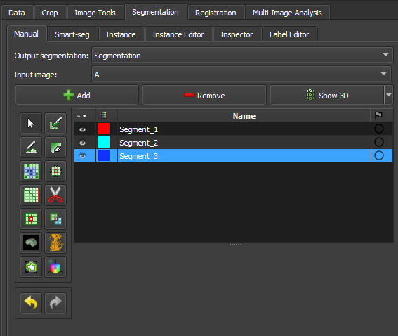
Panels and their usage


Figure 1: Overview of the segment editor module.

Main options

Segmentation: choose the segmentation to be edited.
Source volume: choose the volume to be segmented. The source volume selected the first time after the segmentation is created is used to determine the labelmap representation geometry of the segmentation (extent, resolution, axis directions, origin). The source volume is used by all editor effects that use the intensity of the segmented volume (e.g., threshold, level tracing). The source volume can be changed at any time during the segmentation process.
Add: Add a new segment to the segmentation and select it.
Remove: select the segment you want to delete and click Remove segment to delete it from the segmentation.
Show 3D: display your segmentation in the 3D viewer. This is a toggle button. When enabled, the surface is automatically created and updated as the user segments. When disabled, the conversion is not continuous, and the segmentation process is faster. To change the surface creation parameters: click the arrow next to the button, go to the "Smoothing factor" option, and use the value bar to edit a conversion parameter value. Setting the smoothing factor to 0 disables smoothing, making updates much faster. Set the smoothing factor to 0.1 for weak smoothing and 0.5 or higher for stronger smoothing.

Segments Table

This table displays the list of all segments.

Table columns:

Visibility (eye icon): Toggles segment visibility. To customize the display: open slice display controls (click the double-arrow button icons at the top of a slice viewer) or go to the Segmentations module.
Color swatch: set the color and assign the segment to standardized terminology.
Status (flag icon): This column can be used to set the editing status of each segment which can be used to filter the table or mark segments for further processing. Not started: default initial state, indicates that editing has not yet occurred. In progress: when a “not started” segment is edited, its status is automatically changed to this. Completed: the user can manually select this state to indicate that the segment is complete. Flagged: the user can manually select this state for any custom purpose, e.g., to draw the attention of an expert reviewer to the segment.

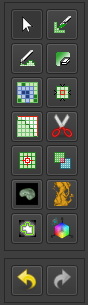
Effects section


Figure 2: Effects section of the segment editor.

Effects toolbar: Select the desired effect here. See below for more information on each effect.
Options: The options for the selected effect will be displayed here.
Undo/Redo: The module saves the state of the segmentation before each effect is applied. This is useful for experimentation and error correction. By default, the last 10 states are remembered.

Effects

Effects operate by clicking the Apply button in the effect's options section or by clicking and/or dragging in the slice or 3D views.

Paint

Choose the radius (in millimeters) of the brush to be applied.
Left-click to apply a single circle.
Left-click and drag to fill a region.
A trail of circles is left, which is applied when the mouse button is released.
Sphere mode applies the radius to slices above and below the current slice.

Draw

Left-click to create individual points of an outline.
Left-drag to create a continuous line of points.
Double left-click to add a point and fill the outline. Alternatively, right-click to fill the current outline without adding more points.

Note

The Scissors effect can also be used for drawing. The Scissors effect works in both slice and 3D views, can be configured to draw on more than one slice at a time, can also erase, can be restricted to drawing horizontal/vertical lines (using rectangle mode), etc.

Erase

Similar to the Paint effect, but the highlighted regions are removed from the selected segment instead of added.

If the Mask / Editable Area is set to a specific segment, the highlighted region is removed from the selected segment and added to the mask segment. This is useful when a part of a segment needs to be separated into another segment.

Level Tracing

Moving the mouse defines an outline where pixels have the same background value as the current background pixel.
Left-clicking applies this outline to the label map.

Grow from Seeds

Draw the segment within each anatomical structure. This method will start from these "seeds" and expand them to achieve the complete segmentation.

Initialize: Click this button after the initial segmentation is completed (using other editor effects). The initial calculation may take longer than subsequent updates. The source volume and automatic fill method will be locked after initialization, so if any of these need to be changed, click Cancel and initialize again.
Update: Update the completed segmentation based on altered inputs.
Auto-update: Enable this option to automatically refresh the result preview when the segmentation is changed.
Cancel: Remove result preview. Seeds are kept unchanged, so parameters can be changed, and segmentation can be restarted by clicking Initialize.
Apply: Replace seed segments with visualized results.

Notes:

Only visible segments are used by this effect.
At least two segments are required.
If a part of a segment is erased or painting is removed using Undo (and not replaced by another segment), it is recommended to cancel and initialize again. The reason is that the effect of adding more information (painting more seeds) can propagate to the entire segmentation, but removing information (removing some seed regions) will not change the complete segmentation.
The method uses an improved version of the grow-cut algorithm described in Liangjia Zhu, Ivan Kolesov, Yi Gao, Ron Kikinis, Allen Tannenbaum. An Effective Interactive Medical Image Segmentation Method Using Fast GrowCut, International Conference on Medical Image Computing and Computer Assisted Intervention (MICCAI), Interactive Medical Image Computing Workshop, 2014.

Margin

Increases or decreases the selected segment by the specified margin.

By enabling Apply to visible segments, all visible segments of the segmentation will be processed (in the order of the segments list).

Smoothing

Smooths segments by filling holes and/or removing extrusions.

By default, the current segment will be smoothed. By enabling Apply to visible segments, all visible segments of the segmentation will be smoothed (in the order of the segments list). This operation can be time-consuming for complex segmentations. The Joint smoothing method always smooths all visible segments.

Clicking the Apply button, the entire segmentation is smoothed. To smooth a specific region, left-click and drag in any slice or 3D view. The same smoothing method and strength are used in both whole-segmentation mode and region-based smoothing mode (brush size does not affect Smoothing strength, it only facilitates designating a larger region).

Available methods:

Median: removes small extrusions and fills small gaps while keeping smooth contours virtually unchanged. Applied only to the selected segment.
Opening: removes extrusions smaller than the specified kernel size. Adds nothing to the segment. Applied only to the selected segment.
Closing: fills sharp corners and holes smaller than the specified kernel size. Removes nothing from the segment. Applied only to the selected segment.
Gaussian: smooths all details. The strongest possible smoothing, but tends to shrink the segment. Applied only to the selected segment.
Joint smoothing: smooths multiple segments at once, preserving the watertight interface between them. If segments overlap, the segment higher in the segments table takes precedence. Applied to all visible segments.

Scissors

Cuts segments to the specified region or fills regions of a segment (often used with masking). Regions can be drawn in both slice view and 3D views.

Left-click to start drawing (freeform or elastic circle/rectangle)
Release button to apply

By enabling Apply to visible segments, all visible segments of the segmentation will be processed (in the order of the segments list).

Islands

Use this tool to process "islands", i.e., connected regions that are defined as groups of non-empty voxels that touch each other but are surrounded by empty voxels.

Keep largest island: keeps the largest connected region.
Remove small islands: keeps all connected regions that are larger than the minimum size.
Split islands into segments: creates a single segment for each connected region of the selected segment.
Keep selected island: after selecting this mode, click on a non-empty area in the slice view to keep that region and remove all other regions.
Remove selected island: after selecting this mode, click on a non-empty area in the slice view to remove that region and preserve all other regions.
Add selected island: after selecting this mode, click on an empty area in the slice view to add that empty region to the segment (fill hole).

Logical Operators

Apply basic copy, clear, fill, and Boolean operations to the selected segment(s). See more details on the methods by clicking “Show details” in the effect description in the Segment Editor.

Mask Volume

Erase inside/outside a segment in a volume or create a binary mask. The result can be saved to a new volume or overwrite the input volume. This is useful for removing irrelevant details from an image or creating masks for image processing operations (such as registration or intensity correction).

Operation:
- Fill inside: sets all voxels of the selected volume to the specified Fill value inside the selected segment.
- Fill outside: sets all voxels of the selected volume to the specified Fill value outside the selected segment.
- Fill inside and outside: creates a binary labelmap volume as output, filled with the Fill outside value and Fill inside value. Most image processing operations require the background region (outside, ignored) to be filled with the value 0.
Smooth border: if set to >0, the transition between inside/outside the mask is gradual. The value specifies the standard deviation of the Gaussian blur function. Larger values result in a smoother transition.
Input volume: voxels from this volume will be used as input for the mask. The geometry and voxel type of the output volume will be the same as this volume.
Output volume: this volume will store the mask result. While it can be the same as the input volume, it is often better to use a different output volume, because then options can be adjusted, and the mask can be recalculated multiple times.

Color Threshold

This segmentation editing effect, called "Color threshold", allows the segmentation of images based on user-defined color ranges. The effect can operate in HSV or RGB color modes, allowing adjustments to hue, saturation, and value components. It also has adjustments for red, green, and blue levels. The effect offers a real-time visualization of the segmentation, using a preview pulse to help the user refine parameters before permanently applying changes. Additionally, the effect includes advanced functionalities, such as color space conversion and manipulation of circular ranges, enabling precise and customized segmentation.

Connectivity

This "Connectivity" effect allows segment selection in Geoslicer, enabling users to calculate connected regions within a segment in a specific direction. The effect includes configurable parameters such as connectivity jumps, direction, and output name, making it a versatile tool for detailed segmentation tasks. It efficiently handles connected component analysis and generates a new segment based on user-defined settings.

Boundary Removal

Removes the borders of visible segments using an edge detection filter. Only visible segments are modified in the process.

Filter: Only gradient magnitude so far.
Threshold adjustment: Adjusts the threshold to find a suitable border.
Keep filter result: Check this option to keep the filter result as a new volume, for inspection.

Expand Segments

Applies the watershed process to expand visible segments, filling the empty spaces of the segmentation. The selected visible segments are used as seeds, or minima, from which they are expanded.

Smart Foreground

Automatically segments the useful area of an image or volume, i.e., the region that actually corresponds to the sample, rejecting border regions. By enabling the fragmentation feature (currently available only for thin sections), any fissures between rock fragments also cease to be considered useful area. This effect is convenient for workflows where areas adjacent to the rock might negatively influence results, such as determining the porosity rate of the sample.

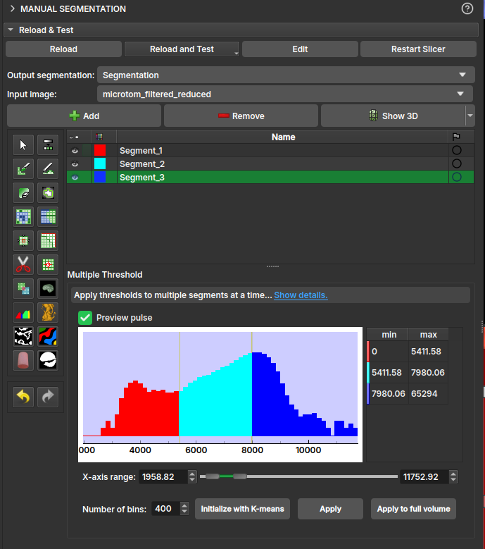
Multiple Thresholds

The multiple threshold effect, available in the Volumes, Image Log, Core, and Multiscale environments, allows the user to segment a 3D volume based on multiple threshold values. Depending on the number of selected segments, a histogram with thresholds appears colored in the interface. Each segment will be separated by the threshold, with the next segment starting at a slightly higher threshold on the grayscale. This way, the image can be easily segmented based on its grayscale values.

Operation:
- Fill internally: segments the entire useful area of the image/volume;
- Erase externally: given any already filled segment, it excludes all its region that resides outside the useful area.
Fragmentation:
- Split: enables/disables the fragmentation feature. Recommended only for polarized light thin section (PP) images. Once enabled, it allows choosing between:
  - Keep all: considers all fragments as useful area;
  - Filter the N largest: only the N fragments with the largest area will be preserved, where N is the value specified by the user.

Automatic Thin Section Segmentation

The segmentation of petrographic thin section images can be done in two ways: binary segmentation, which identifies only the pore phase, and multiphase segmentation, which identifies the various minerals that make up the rock.

Multiphase Segmentation (Minerals)

The analysis of mineral composition and rock texture is fundamental for the petroleum industry. GeoSlicer uses Deep Learning models to automate this analysis from thin section images, offering an alternative to the QEMSCAN method.

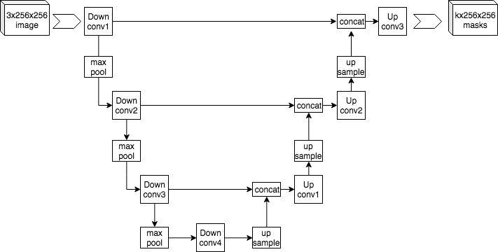
Convolutional Neural Network (U-Net)

For mineralogical segmentation, GeoSlicer employs a convolutional neural network with the U-Net architecture. This type of network is ideal for semantic segmentation, as it assigns a class to each pixel of the image, precisely delimiting the region of each element. The U-Net consists of an encoding path, which extracts features from the image at multiple scales, and a decoding path, which reconstructs the segmentation map.


Figure 1: Example U-Net architecture.

Training

Model training was performed using over 50 high-resolution thin sections, employing Plane Polarized Light (PP) and Cross-Polarized Light (PX) images. The QEMSCAN result was used as a ground truth. PP, PX, and QEMSCAN images were aligned through a registration process, and training focused on a region of interest (SOI) to minimize edge noise. To increase data diversity, thin section cutouts underwent random transformations, such as rotations and inversions. Models were trained to identify Pores and the minerals Calcite, Dolomite, Mg-Clay minerals, Quartz, and a generic Others class.

Results

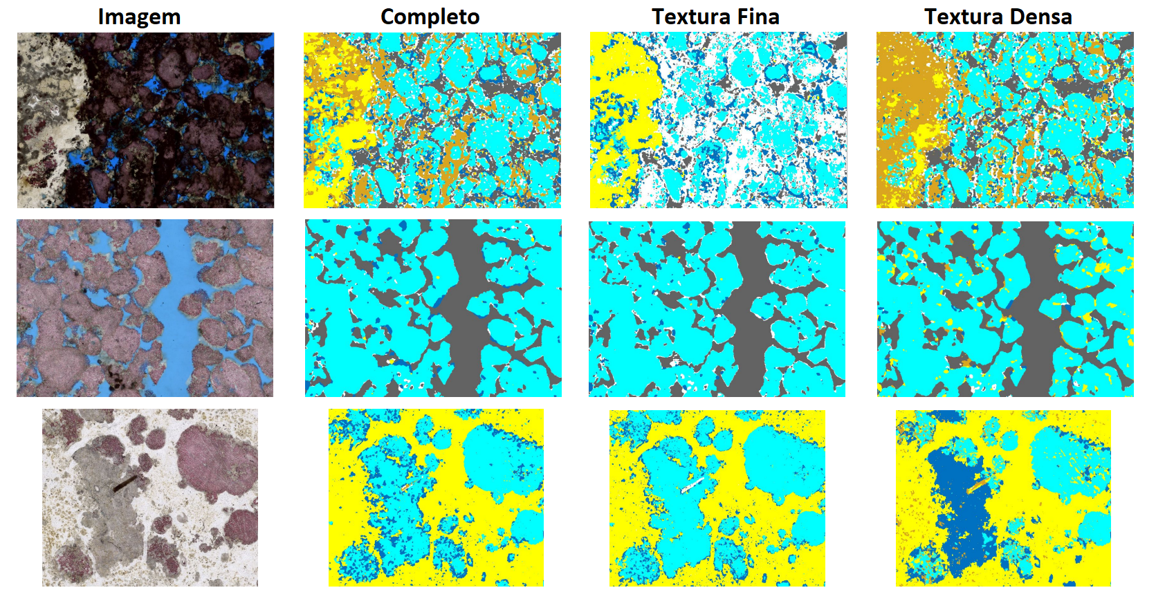
The final models, integrated into GeoSlicer, show good approximations of mineral composition, especially for the study of textures and phase distribution. Below is an example of a prediction on thin sections not seen during training.


Figure 2: Prediction of the final models on unseen thin sections.

Pore/Non-pore Segmentation

Porosity is a crucial indicator of a reservoir's potential. GeoSlicer offers automatic methods for segmenting pores, which are typically filled with blue resin for highlight.

Convolutional Neural Networks (U-Net)

As in multiphase segmentation, the U-Net architecture is used for pore segmentation.

Training

The model was trained with 85 thin section images, where the reference segmentation was obtained by color thresholding on the blue resin. The thin sections were divided into 128x128 pixel cutouts, and only the useful areas (delimited by the SOI) were considered. Training lasted 300 epochs, with random modifications (rotations, inversions) applied to diversify the data and improve the model's generalization capability.

Results

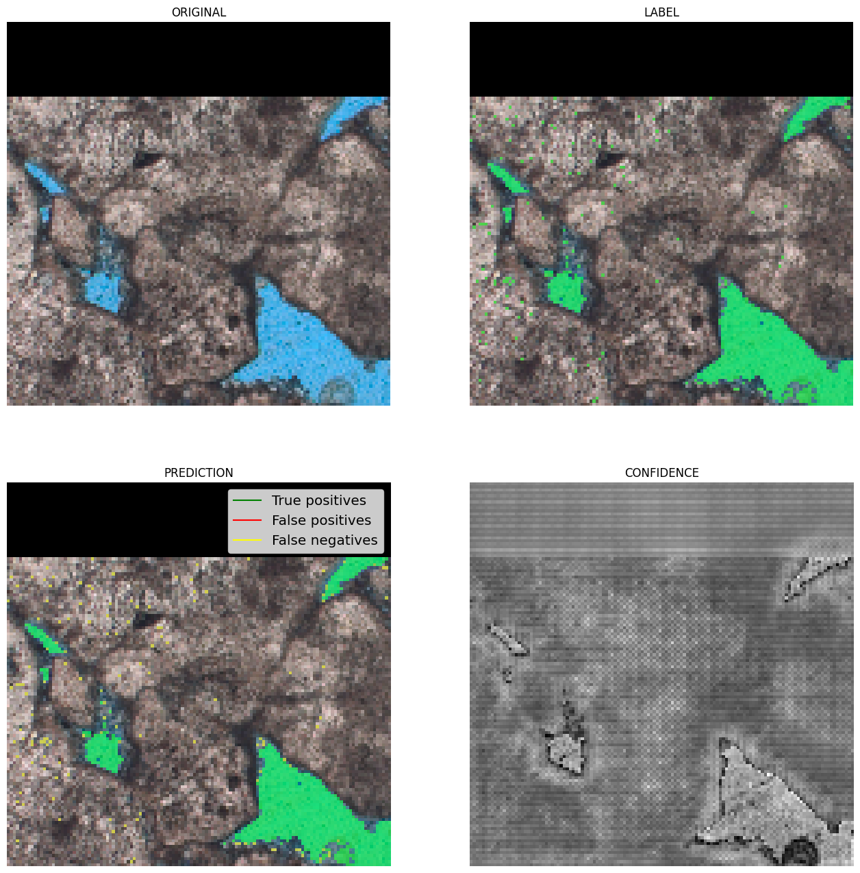
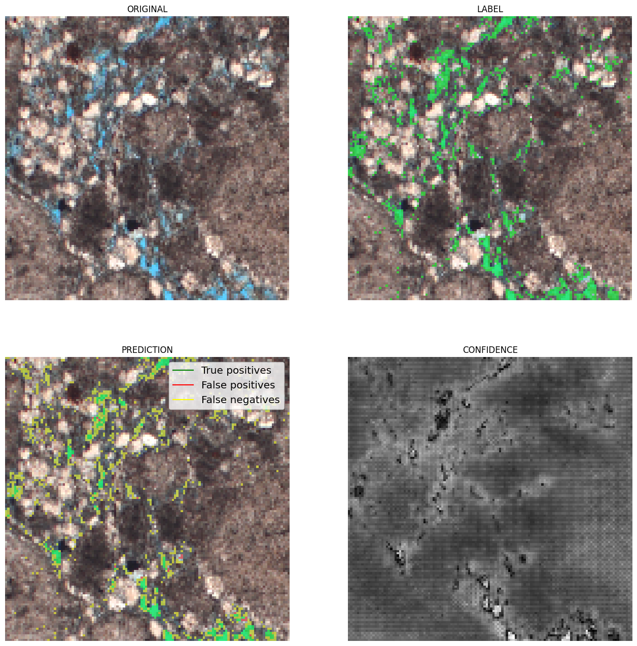
The model achieved satisfactory performance, with a Dice coefficient (overlap) greater than 85%. The results show that the network can identify pores with high confidence, although it may present some difficulties at the edges, where colors are intermediate.


Figure 3: Examples of results. In green, true positives; in red, false positives; and in yellow, false negatives.

Bayesian Inference

As an alternative to neural networks, Bayesian Inference offers a simpler model for pore/non-pore segmentation. This method uses Bayes' rule to calculate the probability of a pixel belonging to a segment (pore or non-pore) based on a mean and a covariance matrix learned during training.

The approach uses a Multivariate Normal Distribution as a likelihood function:

\[ f(x_p|s)=\frac{1}{\sqrt{(2\pi)^k \det \Sigma_s}}\exp\left(-\frac{1}{2}(x_p-\mu_s)^T \Sigma_s^{-1} (x_p-\mu_s)\right) \]

Where \(x_p\) is the pixel vector in a window, and \(\mu_s\) and \(\Sigma_s\) are the mean and covariance of segment \(s\).

Training and Results

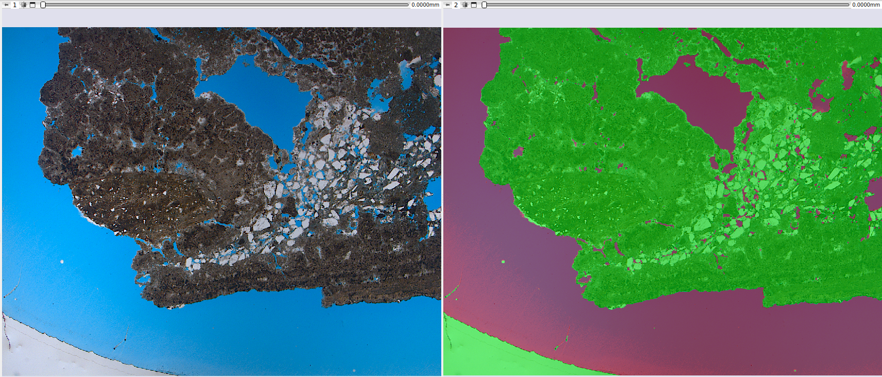
To improve results, thin section images, originally in RGB format, are converted to HSV. The model was trained on a small dataset (~10 samples) and, even with a simple approach, produces interesting results for pore/non-pore segmentation.


Figure 4: Qualitative result of pore/non-pore segmentation by Bayesian inference.

References

DE FIGUEIREDO, L. P. et al. (2020). Direct Multivariate Simulation - A stepwise conditional transformation for multivariate geostatistical simulation. Computers & Geosciences.
DE FIGUEIREDO, L. P. et al. (2017). Bayesian seismic inversion based on rock-physics prior modeling for the joint estimation of acoustic impedance, porosity and lithofacies. Journal of Computational Physics.
HUNT, B. R. (1977). Bayesian methods in nonlinear digital image restoration. IEEE Transactions on Computers.
SKILLING, J. & BRYAN, R. K. (1984). Maximum entropy image reconstruction: general algorithm. Monthly Notices of the Royal Astronomical Society.
HANSON, K. (1993). Introduction to Bayesian image analysis. Proc SPIE.
HANSON, K. (1990). Object detection and amplitude estimation based on maximum a-posteriori reconstructions. Proc. SPIE.
GEMAN, S. & GEMAN, D. (1990). Stochastic Relaxation, Gibbs Distribution and the Bayesian Restoration of Images. IEEE, Transactions on Pattern Analysis; Machine Intelligence.
AITKIN, M. A. (2010). Statistical inference: an integrated Bayesian/likelihood approach. CRC Press.
MIGON, H. S. et al. (2014). Statistical Inference: An Integrated Approach. 2nd ed. CRC Press.
GAMERMAN, D. & LOPES, H. F. (2006). Monte Carlo Markov Chain: Stochastic Simulation for Bayesian Inference. 2nd ed. Chapman & Hall.

Segment Inspector

This module provides several methods to analyze a segmented image. Particularly, the Watershed and Separate Objects algorithms allow a segmentation to be fragmented into multiple partitions, or multiple segments. It is generally applied to the segmentation of porous space to calculate the metrics of each porous element. The input is a segmentation node or labelmap volume, a region of interest (defined by a segmentation node), and the master image/volume. The output is a labelmap where each partition (pore element) is in a different color, a table with global parameters, and a table with the different metrics for each partition.

Panels and their use


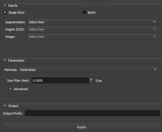
Figure 1: Overview of the Segment Inspector module.

Main options

The Segment Inspector module interface is composed of Inputs, Parameters, and Output.

Single input


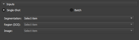
Figure 2: Overview of the inputs in the Segment Inspector module.

Segmentation: Input for the segmentation used in the partition.
Region SOI: Choose a segmentation of interest that contains at least part of the segmentation used in Segmentation.
Image: Field automatically filled with the reference node of the segmentation used in Segmentation.

Attributes


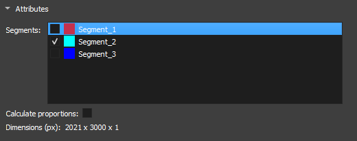
Figure 3: Segment attributes in the Segment Inspector module.

Segments: Segments contained in the segmentation selected in Segmentation. The list shows the visualization of the segment via the eye icon. For the fragmentation method to be initialized, a segment must be selected.
Calculate proportions: Checkbox to display the proportions of each segment in the image.
Dimension(px): Displays the dimensions of the selected image.

Parameters and Methods

Watershed

The Watershed algorithm works by simulating the expansion of "watersheds" from points marked as local minima. As "water" fills the valleys, it defines the boundaries between different regions. This approach is widely used in applications where it is necessary to separate objects or pores in materials, taking advantage of contrasts between regions.


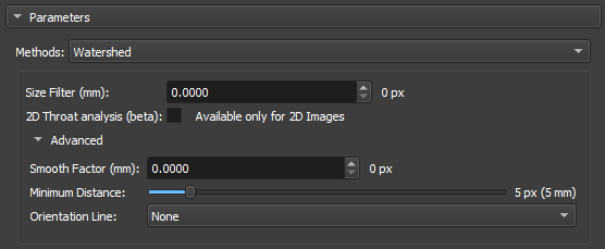
Figure 4: Watershed in the Segment Inspector module.

Size Filter(mm): Controls the maximum segmentation range, directly influencing the size and connectivity of the segmented regions. Small values are used when you want to segment many fine details, whereas large values are used when the focus is on large areas or connected objects.
2D throat analysis(beta): Adds 2D throat analysis metrics to the report.
Calculate Coordination Number: Calculates the number of neighboring regions (that share a border) with each of the watershed labels. We consider as a "neighbor" any label that shares a face, edge or vertex of another nearby.
Smooth factor: Parameter that adjusts the degree of smoothness on the edges of segmented regions, allowing control between preserving details and reducing noise or irregularities. With high factors, the segmentation will be smoother and simplified, but with loss of small details.
Minimun Distance: parameter that determines the smallest allowed distance between two local maxima or segmented objects. A larger value for this parameter will merge nearby objects, simplifying the segmentation, while a smaller value will allow the separation of closer objects, resulting in a more detailed segmentation.
Orientation Line: The orientation parameter allows the algorithm to align itself properly with the image features, improving segmentation accuracy.

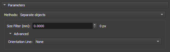
Separate Objects

The "Separate Objects" segmentation method identifies connected regions in a binary matrix that represent information objects. This process is especially useful in porosity analysis, where it is important to distinguish different connected regions within a volume.


Figure 5: Separate Objects in the Segment Inspector module.

Size Filter(mm): Controls the maximum segmentation range, directly influencing the size and connectivity of the segmented regions. Small values are used when you want to segment many fine details, whereas large values are used when the focus is on large areas or connected objects.
Orientation Line: The orientation parameter allows the algorithm to align itself properly with the image features, improving segmentation accuracy.

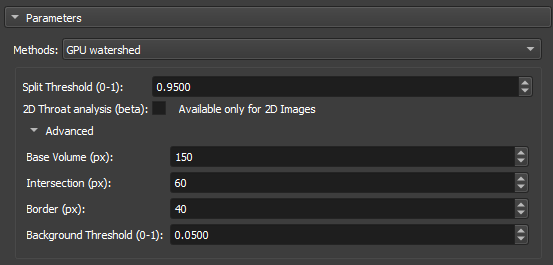
GPU Watershed

The Deep Watershed technique combines the traditional Watershed concept with deep neural networks to obtain more precise and robust segmentation. Using the power of deep learning, the method enhances the detection of boundaries and objects in complex scenarios, such as the analysis of porous materials with multiple levels of overlap. This approach is particularly effective for handling three-dimensional volumes and for performing precise segmentations in noisy images.


Figure 6: GPU Watershed in the Segment Inspector module.

Split Threshold(0-1): Controls the maximum segmentation range, directly influencing the size and connectivity of the segmented regions. Small values are used when you want to segment many fine details, whereas large values are used when the focus is on large areas or connected objects.
2D throat analysis(beta): Adds 2D throat analysis metrics to the report.
Base volume (px): This parameter represents a base value that can be related to the size or scale of the volume being processed. It serves as a reference for calculating the depth or layers of the volume that will be analyzed.
Intersection (px): This parameter is used to adjust how much regions within the volume can overlap during segmentation.
Border (px): This parameter defines the size or thickness of the borders that will be considered when calculating the depth layers in the volume.
Background Threshold(0-1): Acts as a cutoff point. All values below this threshold are considered to belong to the background, while values above the threshold are considered to be parts of objects or significant regions within the image or volume.

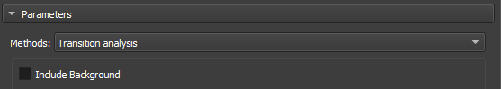
Transitions Analysis

Transitions Analysis focuses on examining the changes between regions or segments of an image. This method is mainly employed to study the mineralogy of samples.


Figure 7: Transitions Analysis in the Segment Inspector module.

Include Background: Uses the total dimensions of the input image for analysis.

Basic Petrophysics


Figure 8: Transitions Analysis in the Segment Inspector module.

Include Background: Uses the total dimensions of the input image for analysis.

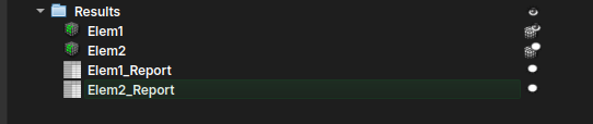
Output

Enter a name to be used as a prefix for the results object (labelmap where each partition (pore element) is in a different color, a table with global parameters, and a table with the different metrics for each partition).

Properties / Metrics:

Label: partition label identification.
mean: mean value of the input image/volume within the partition region (pore/grain).
median: median value of the input image/volume within the partition region (pore/grain).
stddev: Standard deviation of the input image/volume value within the partition region (pore/grain).
voxelCount: Total number of pixels/voxels in the partition region (pore/grain).
area: Total area of the partition (pore/grain). Unit: mm².
angle: Angle in degrees (between 270 and 90) related to the orientation line (optional, if no line is selected, the reference orientation is the upper horizontal).
max_feret: Major Feret diameter. Unit: mm.
min_feret: Minor Feret diameter. Unit: mm.
mean_feret: Average of the minimum and maximum axes.
aspect_ratio: min_feret / max_feret.
elongation: max_feret / min_feret.
eccentricity: square(1 - min_feret / max_feret), related to the equivalent ellipse (0 ≤ e < 1), equal to 0 for circles.
ellipse_perimeter: Perimeter of the equivalent ellipse (equivalent ellipse with axes given by the minimum and maximum Feret diameters). Unit: mm.
ellipse_area: Area of the equivalent ellipse (equivalent ellipse with axes given by the minimum and maximum Feret diameters). Unit: mm².
ellipse_perimeter_over_ellipse_area: Perimeter of the equivalent ellipse divided by its area.
perimeter: Actual perimeter of the partition (pore/grain). Unit: mm.
perimeter_over_area: Actual perimeter divided by the area of the partition (pore/grain).
gamma: Circularity of an area calculated as 'gamma = perimeter / (2 * square(PI * area))'.
pore_size_class: Pore class symbol/code/id.
pore_size_class_label: Pore class label.

Definition of pore classes:

Micropore: class = 0, max_feret less than 0.062 mm.
Very small mesopore: class = 1, max_feret between 0.062 and 0.125 mm.
Small mesopore: class = 2, max_feret between 0.125 and 0.25 mm.
Medium mesopore: class = 3, max_feret between 0.25 and 0.5 mm.
Large mesopore: class = 4, max_feret between 0.5 and 1 mm.
Very large mesopore: class = 5, max_feret between 1 and 4 mm.
Small megapre: class = 6, max_feret between 4 and 32 mm.
Large megapre: class = 7, max_feret greater than 32 mm.

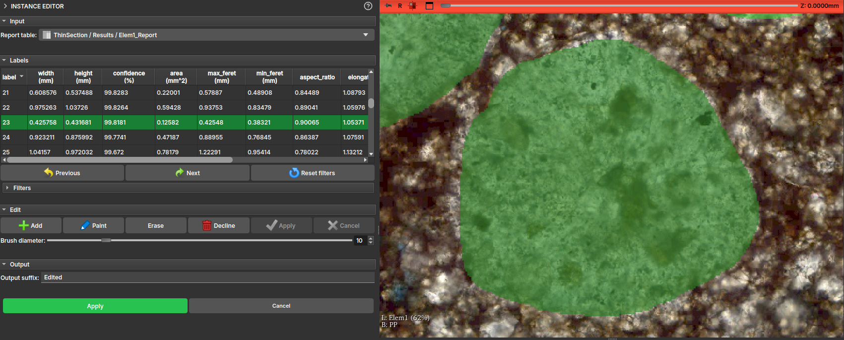
Instance Editor

This module is used to manipulate and perform a label-by-label inspection of the results generated from an "Textural Structures" model of the AI Segmenter. When using the AI Segmenter module with this model on a thin section image, the result should be something like:

inputs

After the instance segmentation results are generated, the user might want to repaint, clean, or even inspect each of the created instances. Therefore, when loading one of the Report tables into the Instance Editor module, it should automatically display the LabelMap volume associated with the table.

modulo

Tip

An opacity for the labels can be chosen to better visualize the sample beneath them. One practical way to do this is by holding the Ctrl button and dragging the mouse horizontally while clicking inside the viewing window.

The module interface will display a table with the main properties of the drawing, and the user can then, by clicking on the table entries or using the Next and Previous buttons, visit each of the elements individually.

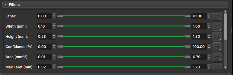
Additionally, the interface features a Filters tool that lists all properties and allows selecting a certain range of these properties, applying a color to the table elements and enabling the user to more easily decide whether to keep or delete that element.

filtros

In the Edit field, some label editing tools are presented, including: - Add: Adds a new instance/label to the table, allowing the user to draw freehand over the thin section view; - Paint: Activates a brush tool, to use on an existing instance; - Erase: Activates an eraser tool, to erase part of an existing instance; - Decline: Deletes the instance entry from both the table and the drawing; - Apply: Applies the current change, recalculating the drawing properties; - Cancel: Discards the current change;

Info

All changes made are temporary; to apply them and generate a new table and a new LabelMap with the drawings, it is necessary to finalize the changes by pressing the general "Apply" button, available further down in the interface.

LabelMap Editor

This module allows the editing of labelmaps, typically generated by the Watershed algorithm in the Segment Inspector module.

The results generated by the watershed are not always as expected; this module allows the user to edit these results label-by-label, merging or splitting the divisions made by the algorithm.

module

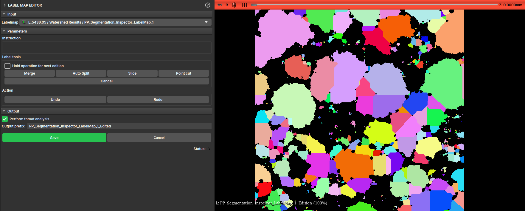
The module features an interface with the following operations:

Merge: Merges two labels;
Auto Split: Attempts to split a label into more than one part;
Slice: Cuts the label along a user-defined line;
Point cut: Cuts the label along a line passing through a user-defined point;

The interface also features Undo and Redo buttons to revert or advance changes.

Pore Stats: statistics and properties of pores and particles in thin section

The Pore Stats module offers features for calculating geological properties of pores in batches of rock thin section images, as well as related descriptive statistics. Given an input directory containing images related to the same well, the module is able to segment the porous region, separate the different pores, calculate different properties for each, and save reports and images summarizing the results.

Interface and Functionality

The module is available in the Thin Section environment, under the Segmentation tab, Pore Stats sub-tab. Figure 1 illustrates a general overview of the module's workflow, while Figure 2 shows the module's interface in GeoSlicer and, for each feature, points to the subsection of this section that describes it.


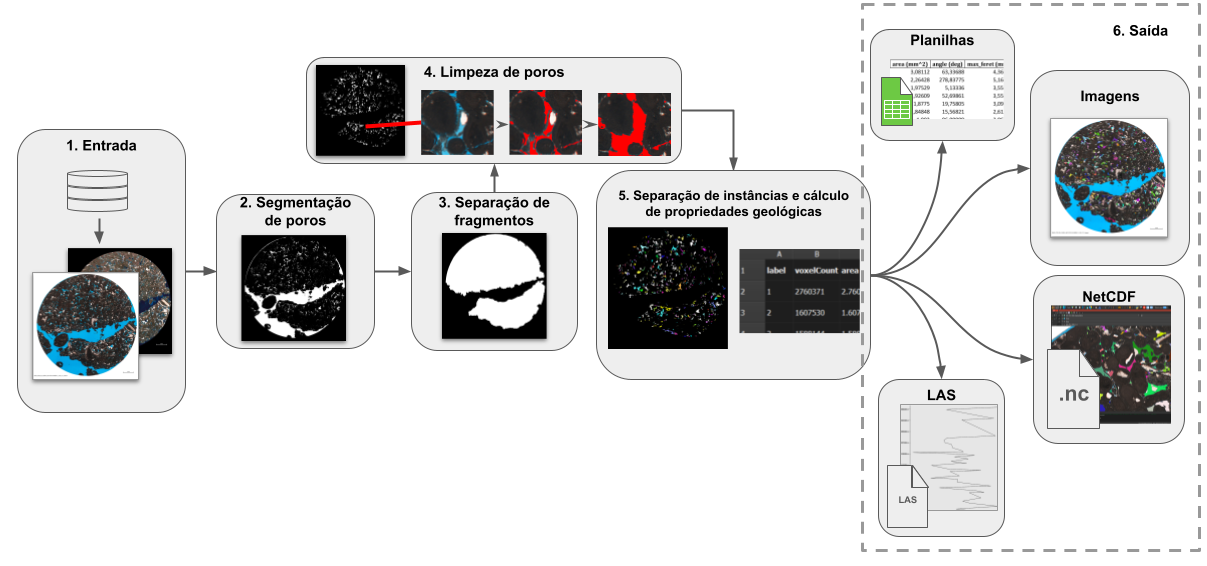Figure 1: General overview of the module's workflow.


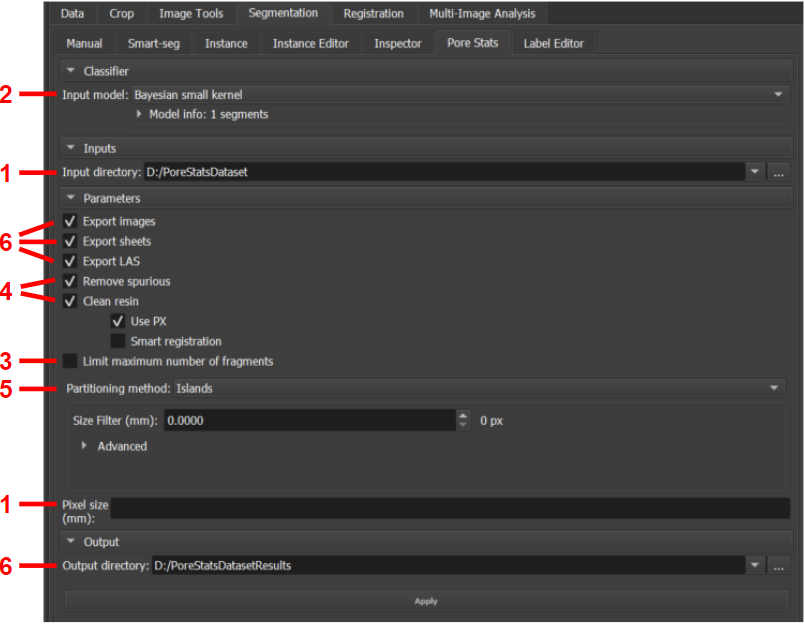
Figure 2: Pore Stats module.

1. Input

The module is designed to iterate over all valid images it finds in a given input directory. An image is considered valid if the file format is PNG, JPEG, or TIFF and its name follows the pattern: <well>_<depth-value>(-optional-index)<depth-unit>_<…>_c1.<extension>. The c1 suffix refers to plane-polarized (PP) images. Optionally, cross-polarized (PX) counterparts found in the same directory can also be used to assist in specific operations, and should have the c2 suffix. An example of an input directory follows:

Diretório_entrada
    |__ ABC-123_3034.00m_2.5x_c1.jpg
    |__ ABC-123_3034.00m_2.5x_c2.jpg
    |__ ABC-123_3080.0-2m_c1.jpg
    |__ ABC-123_3080.0-2m_c2.jpg
    |__ ABC-123_3080.0m_c1.jpg
    |__ ABC-123_3080.0m_c2.jpg
    |__ ABC-123_3126.65m_2.5x_TG_c1.jpg
    |__ ABC-123_3126.65m_2.5x_TG_c2.jpg

The example describes an input directory with 4 JPEG images of well "ABC-123", corresponding to depths of 3034, 3080, and 3126.65 meters, in both PP/c1 and PX/c2 versions. Since there are two variations corresponding to the same depth (3080m), an optional index ("-2") is included in one of them. Between the depth and polarization information, some additional information may exist between underlines (such as "_2.5x_" and "_TG_").

In addition to the input directory, it is also necessary to specify the image scale in mm, that is, how many mm are represented by the distance between one pixel and the subsequent pixel.

The input directory can be defined using the Input directory selector in the module's interface, within the Inputs section of the interface. The image scale must be specified in the Pixel size (mm) field, in the Parameters section.


Figure 3: Input directory selector.


Figure 4: mm/pixel scale field.

2. Pore Segmentation

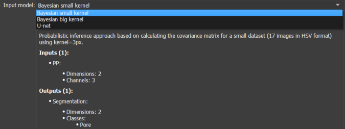
Once an image is loaded, its porous region is segmented using the pre-trained models available in GeoSlicer. In this module, 3 models are available:

Small kernel Bayesian model;
Large kernel Bayesian model;
U-Net convolutional neural model.

Choose the model using the Input model selector in the Classifier section. The information box below the selector can be expanded for more details about each model.


Figure 5: Pore segmentation model selector.

3. Fragment Separation

Many images have large "empty" regions, filled with pore resin, which are detected by the segmenter but do not actually correspond to the rock's porosity, but only to the region around its fragment(s) (see example in Figure 1). In some cases, not all but only the N largest fragments of the rock section are of interest. To isolate the useful rock fragments, the following sequence of operations is applied:

First, the largest fragment, corresponding to the entire area of the section, is isolated from the image edges;
Then, all detected porosity that touches the image border is also discarded, as it is interpreted as visible pore resin around the useful rock area;
Finally, if only the N largest fragments are of interest, the size (in pixels) of each fragment of the remaining useful area is measured and only the N largest are kept.

The module performs fragment separation automatically. However, it is possible to limit the analysis to the N largest by checking the Limit maximum number of fragments checkbox, in the Parameters section, and defining the value of N (between 1 and 20).


Figure 6: Fragment limiter to be analyzed, from largest to smallest.

4. Pore Cleaning

This algorithm is responsible for applying two "cleaning" operations to conventional pore segmentation, which if not performed can negatively impact the final results.

Removal of spurious pores

Current GeoSlicer pore segmenters tend to generate spurious detections in small regions comprising rock but which, due to lighting/resolution/related effects, have a color similar to that of blue pore resin. The module executes a model capable of recognizing these detections and differentiating them from the correct ones, based on pixel values within an interval around the centroid of each segment. All detected spurious pores are discarded.

Incorporation of bubbles and residues into the pore resin

It is common for air bubbles and related residues to form in the pore resin. Segmenters do not detect these artifacts, not interpreting them as pore area, which influences the size and quantity of detected pores. This module aims to "clean" the resin, including these bubbles and residues into the corresponding pore body. Basically, some criteria must be met for an image region to be interpreted as a bubble/residue:

Having white color or blue color with low intensity and saturation: generally, bubbles are white or, when covered with material, have an almost black shade of blue. Residues that eventually surround bubbles also have a low intensity blue level;
Touching the pore resin: the transition between the resin and the artifacts is normally direct and smooth. Since the pore segmentation model accurately detects the resin region, the artifact needs to touch this region. Consequently, the current algorithm cannot detect less common cases where the artifact occupies 100% of the pore area;
Being barely visible in the PX/c2 image (if available): some rock elements may resemble artifacts and also be in contact with the resin. However, generally, artifacts are barely or not at all visible in PX/c2 images, while other elements are usually noticeable. This criterion is more effective the better the registration (spatial alignment) between the PP and PX images. The algorithm attempts to automatically correct image registration by aligning image centers. This step can be preceded by an operation to crop the useful rock area, discarding excess borders.

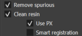
Cleaning operations are recommended, but they can take some time. Therefore, it is possible to disable them by unchecking the Remove spurious checkbox for spurious pore removal and Clean resin for resin cleaning, in the Parameters section. If the latter is enabled, two other options are available:

Use PX to use the PX image for criterion 3 analysis;
Smart registration for automatic decision on whether to perform cropping before automatic registration. Not recommended if images are already naturally registered.


Figure 7: Options for cleaning spurious pores and artifacts in pore resin

5. Instance Separation and Geological Property Calculation

Once the porous region is properly segmented and "cleaned", GeoSlicer's Partitioning feature is used to separate the segmentation into different pore instances and calculate the geological properties of each. The following properties are computed:

Area (mm²);
Angle (°);
Maximum Feret's diameter (mm);
Minimum Feret's diameter (mm);
Aspect ratio;
Elongation;
Eccentricity;
Ellipse perimeter (mm);
Ellipse area (mm²);
Ellipse: perimeter over area (1/mm);
Perimeter (mm);
Perimeter over area;
Gamma.

Within the Parameters section, choose the separation method using the Partitioning method selector, between the Islands option for separation by simple pixel connectivity and Over-Segmented Watershed for applying the SNOW algorithm. Both options allow extra filtering of spurious detections by choosing an acceptable minimum value (Size Filter (mm)) for the size of the major axis (Feret's diameter) of the detection. The watershed selection provides the following extra options:

2D Throat analysis (beta): checkbox that allows including pore throat analysis in the inspection output reports;
Smooth Factor (mm): factor that regulates the creation of more or fewer partitions. Small values are recommended;
Minimum Distance: standard minimum distance between segmentation peaks (points furthest from the edges) to be considered as belonging to different instances.


Figure 8: Options for separating the porous region into different pore instances and calculating their geological properties.

After all input parameters and options are defined, press the Apply button to generate the results.

6. Output

An output directory must also be specified. In it, a pores sub-directory is created, within which a folder is created for each processed image, inheriting the image's name. Inside this folder, three files are created:

AllStats_<image-name>_pores.xlsx: spreadsheet containing the values of the geological properties of each detected instance;
GroupsStats_<image-name>_pores.xlsx: groups detected instances by area similarity and provides various descriptive statistics calculated on the properties of these groups;
<image-name>.png: image that highlights the detected instances in the original image by coloring them randomly.

In each sub-directory, a LAS folder is also created, containing .las files that summarize descriptive statistics of the instances for the entire well, separated by depth.

Finally, netCDF images of the results are also generated. They will be contained in the netCDFs sub-directory.

Example:

Diretório_saída
    |__ pores
    |   |__ LAS
    |   |   |_ las_max.las
    |   |   |_ las_mean.las
    |   |   |_ las_median.las
    |   |   |_ las_min.las
    |   |   |_ las_std.las
    |   |__ ABC-123_3034.00m_2.5x_c1
    |   |   |__ AllStats_ABC-123_3034.00m_2.5x_c1_pores.xlsx
    |   |   |__ GroupsStats_ABC-123_3034.00m_2.5x_c1_pores.xlsx
    |   |   |__ ABC-123_3034.00m_2.5x_c1.png
    |   |__ ...
    |__ netCDFs
        |__ ABC-123_3034.00m_2.5x_c1.nc
        |__ ...

Define the output directory using the Output directory selector in the Output section. If it does not exist, the directory is automatically created.


Figure 9: Output directory selector.

Choose whether or not to generate the output reports using the Export images, Export sheets, and Export LAS checkboxes in the Parameters section. If checked, they respectively ensure the generation of the image illustrating the instances, the property and statistics spreadsheets, and the LAS files describing the well.


Figure 10: Optional export of detected instance illustrations, property and statistics spreadsheets, and LAS files for statistics by depth.

Self-Guided Segmentation (Unsupervised)

The Self-Guided Segmentation module performs unsupervised segmentation of a 2D image. This module is particularly useful for thin section images. It uses a superpixel algorithm along with a simple neural network to segment the image.

SelfGuidedSegmentation

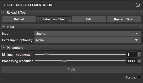
Inputs

Input: A vtkMRMLVectorVolumeNode representing a color image with 3 RGB or HSV channels.
Extra Input (optional): An additional vtkMRMLVectorVolumeNode with 3 channels, which can be used as extra input for the segmentation process. This is useful for incorporating data from other imaging modalities, such as PP/PX images.

Parameters

Minimum segments: This slider determines the minimum number of segments the algorithm will produce. The algorithm will stop if it finds fewer segments than this value.
Processing resolution: This slider controls the resolution at which the segmentation is performed. The image height is reduced to the specified number of pixels for processing, and the resulting segmentation is then scaled up to the original image size. This allows for faster processing at the cost of some detail.

Output

Output segmentation: The module generates a vtkMRMLSegmentationNode containing the segmented image. Each segment is assigned a distinct color for easy visualization.
Merge visible segments: This button allows merging all currently visible segments into a single segment. This is useful for combining multiple segments that belong to the same region of interest.

Fluxos

Segment Editor

The Segment editor module to segment an image, as described in the steps below:

Video: Manual Segmentation

Enter the manual segmentation section of the environment.
Select create new segmentation in Output segmentation.
Select a reference image in Input image.
Click Add to add the number of segments.
The visibility (eye icon), color, and name of the segments can be changed in the segments table.
Select the desired effect from the left-side menu next to the segments table; in the video, color threshold and paint are used.
Parametrize the desired effect and choose the region to be segmented.
Click Apply and wait for completion. A segmentation node will appear, and its visualization can be changed in the Explorer.

Segmenter

Segmenter module for automatically segmenting an image, as described in the steps below:

Go to the Smart-seg segmentation section of the environment.
Select the Pre-trained models.
The Carbonate Multiphase(Unet) model was used as an example.
Check Model inputs and outputs.
Select a previously created SOI (Segment of interest) for the Region SOI parameter.
Select a PP (Plane polarized light) image for the PP parameter.
Select a PX (Crossed polarized light) image for the PX parameter.
A prefix for the resulting segmentation name is generated, but this can be modified in the Output Prefix area.
Click Apply and wait for it to finish. A segmentation node will appear, and its visualization can be changed in the Explorer.

Video: Automatic segmentation with pre-trained model

Smart Foreground

The Smart foreground effect to segment the useful area of the sample in an image or volume. The step-by-step usage is divided into two stages:

Operation: considers useful all areas of the image/volume that do not correspond to the edges.
Fragmentation (optional): eventual fissures between sample fragments are also no longer considered useful area. Available only for 2D images (thin sections) and recommended only for plane-polarized light (PP) thin sections.

Operation

Video: Smart Foreground. Thin section adapted from [Luo *et al.*, 2022](https://onlinelibrary.wiley.com/doi/10.1155/2022/8328764) ([CC BY 4.0](https://creativecommons.org/licenses/by/4.0/)).

Define the input image and output segmentation according to the Segment Editor usage tutorial. Creating segmentation/segments is not necessary if you prefer to edit existing segments.
Select the Smart foreground effect.
Select the segment to which the operation will be applied.
Under Operation, select one of the operations:
- Fill inside: fills the segment over the useful area of the sample.
- Erase outside: excludes already segmented areas over the non-useful area of the sample.
If you wish to apply fragmentation (if available), proceed with the steps below. Otherwise, ensure that the Fragments section (below Operation) is unavailable or that the Split option is unchecked, click Apply and wait for the process to finish.

Fragmentation

Under Fragments, check the Split option.
Select one of the options:
- Keep all: keeps all fragments.
- Filter the largest: keeps only the fragments with the largest area. Enter the number of fragments to preserve.
If you use the public version of GeoSlicer, an Annotations field should be visible, and the following steps should be executed. Otherwise, skip this step.
- Add two new segments to the output segmentation. Alternatively, you can create a new segmentation with two segments.
- Select one of the new segments created. Use marking effects such as Draw, Paint, or Scissors to mark small samples of the rock texture.
- Select the other new segment. Now mark small samples of the pore resin in the image.
- Return to the Smart foreground effect and re-select the segment to which the operation will be applied.
- Under Annotations, select the segmentation that contains the marked segments.
- Under Texture samples and Resin samples, select the segments that mark, respectively, the texture and the resin.
Click Apply and wait for the process to finish.