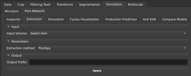
Extractor
This module is used to extract the pore and bond network from: an individualized segmentation of pores (Label Map Volume) performed by a watershed algorithm, generating a uniscalar network; or from a porosity map (Scalar Volume), which will generate a multiscalar model with resolved and unresolved pores.
 |
|---|
| Figure 1: Extraction Module Interface. |
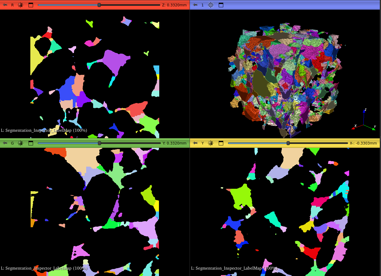
After extraction, the following will be available in the GeoSlicer interface: the pore and throat tables, as well as the network visualization models. The generated tables will be the data used in the subsequent simulation step.
  |
|---|
| Figure 1: On the left, the Label Map used as input for extraction, and on the right, the extracted uniscalar network. |
  |
|---|
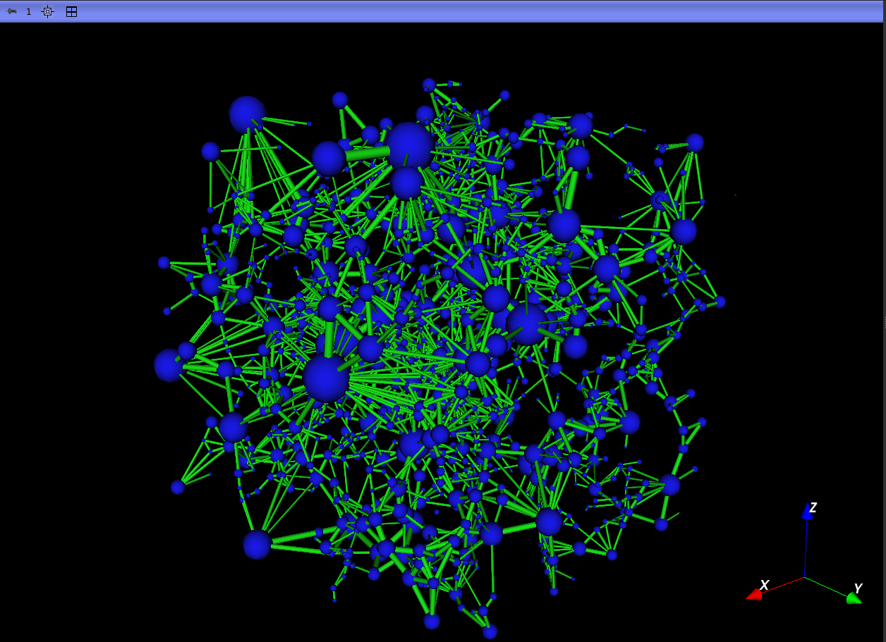
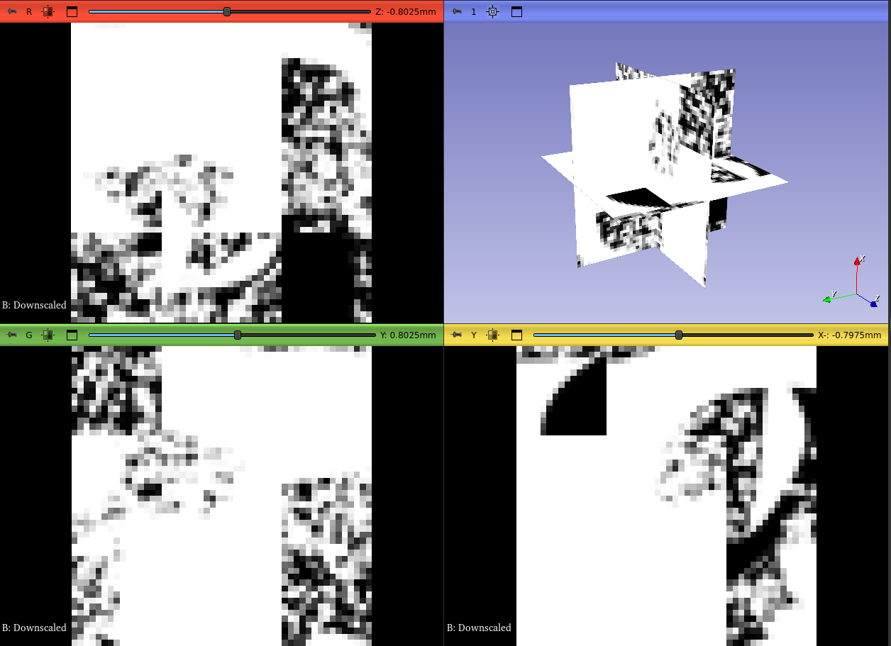
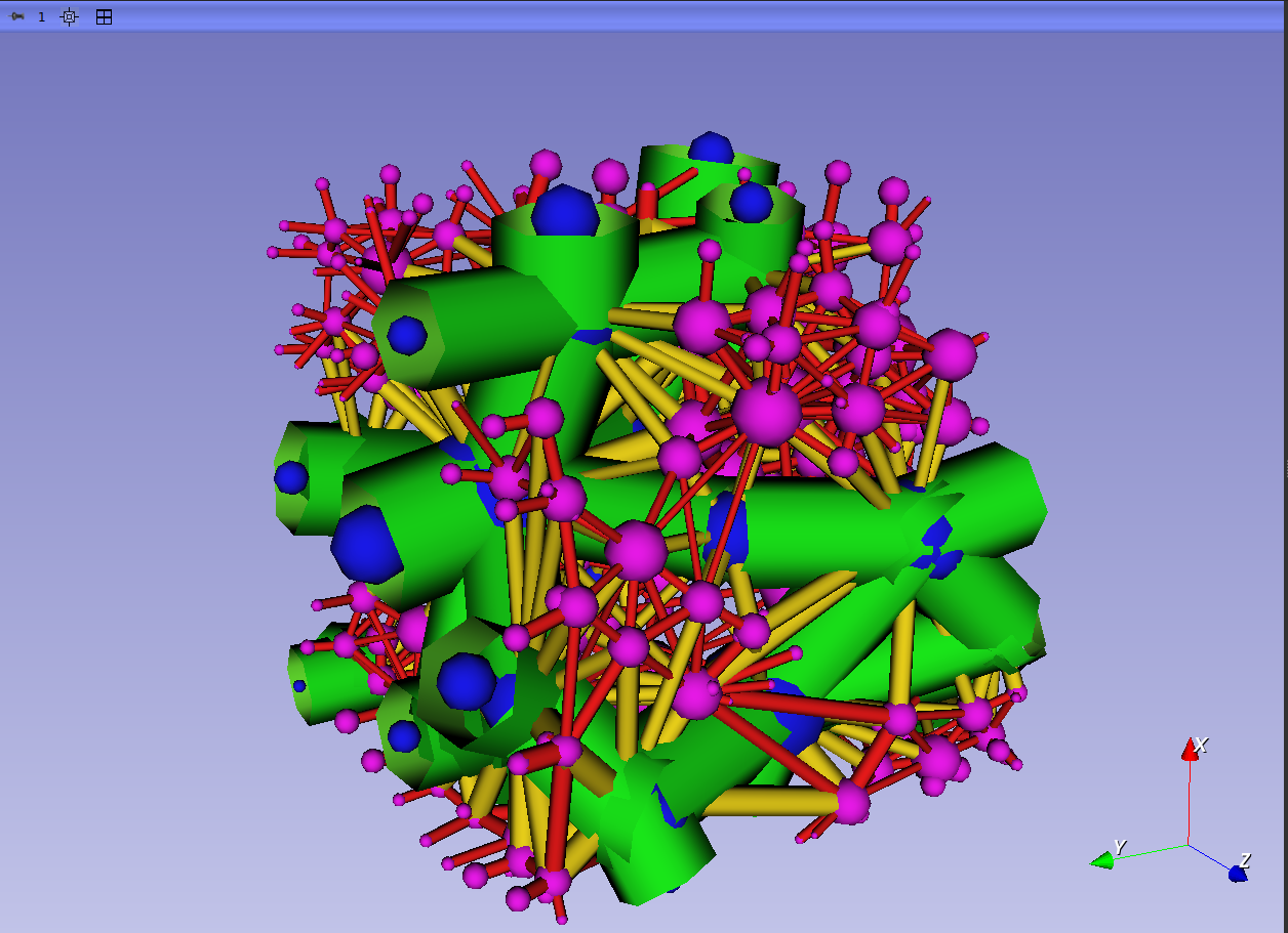
| Figure 2: On the left, the Scalar Volume used as input for extraction, and on the right, the extracted multiscalar network, where blue represents resolved pores, and pink represents unresolved pores. |
Color Scale:
Spheres (Pores):
- Blue - Resolved pore
- Magenta - Unresolved pore
Cylinders (Throats):
- Green - Throat between resolved pores
- Yellow - Throat between a resolved and an unresolved pore
- Red - Throat between unresolved pores
Simulation
This module can perform different types of simulations based on the results of the pore and connection table (created in the [Extraction] module). The simulations include: One-phase, Two-phase, Mercury injection, explained in the following sections.
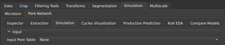
All simulations have the same input arguments: The pore table generated from the network extraction and, when the volume is multiscale, the subscale model used and its parameterization.
 |
|---|
| Figure 1: Input of the pore table generated with the Extraction module. |
One-phase
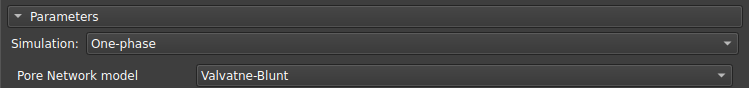
The one-phase simulation is mainly used to determine the absolute permeability (\(K_{abs}\)) property of the sample.
 |
|---|
| Figure 2: Single-phase simulation. |
Three different solvers can be used for this type of simulation:
- pypardiso (recommended): yields the best results, converging even in situations with very discrepant radii;
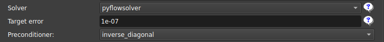
- pyflowsolver: includes an option to select the stopping criterion, but with lower performance than pypardiso;
- openpnm: the most traditionally used option;
 |
|---|
| Figure 3: Pyflowsolver option and stopping criterion. The other options (pypardiso and openpnm) do not have this criterion. |
When the conductivity values are very different for the same sample, and this sample percolates more through the subscale, we may have problems converging to the solution. Because of this, we added an option to limit the values at high conductivities.
 |
|---|
| Figure 4: Options for limiting conductivity values. |
In addition, single-phase simulation can be performed in a single direction or in multiple directions using the Orientation scheme parameter.
 |
|---|
| Figure 5: Orientation scheme used. |
Two-phase
The two-phase simulation consists of initially injecting oil into the sample and increasing its pressure so that it invades virtually all pores, in a process known as drainage. After this first stage, the oil is replaced with water and the pressure is increased again to allow the water to invade some of the pores that were previously filled with oil, expelling the latter. This second process is known as imbibition. By measuring the permeability of the rock in relation to absolute permeability, as a function of water saturation during this process, we obtain the curve known as the relative permeability curve (\(K_{rel}\)).
Since each rock can interact physically or chemically with oil and water in different ways, we need a fairly large variety of parameters to calibrate the results in order to model and simplify this interaction, so that we can extract some physical meaning from the rock properties from the simulation. Below, we list some parameters that can be found in the two-phase simulation available in GeoSlicer.
Currently, we have two algorithms available in GeoSlicer to perform two-phase simulation. The first is PNFlow, which is a standard algorithm implemented in C++, and the second is an algorithm developed by LTrace in Python.
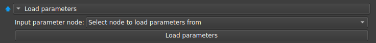
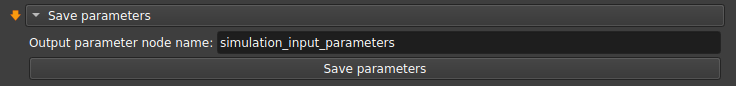
Save/Load parameter selection table
To facilitate the reproduction of simulations that run on the same set of parameters, the interface has options to save/load parameters from tables that are saved with the project. Thus, when calibrating the set of parameters, the user can save this information for later analysis or use these same parameters in another sample.
  |
|---|
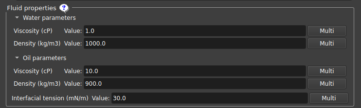
Fluid properties
In this section, you can change the parameters of the fluids (water and oil) used in the simulation:
 |
|---|
| Figure 7: Input of fluid parameters (water and oil). |
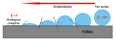
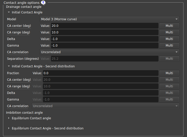
Contact angle options
One of the main properties that affect the interaction of a liquid with a solid is wettability, which can be determined from the contact angle formed by the former when in contact with the latter. Thus, if the contact angle is close to zero, there is a strong interaction that “binds” the liquid to the solid, whereas when the contact angle is close to 180°, the interaction of the liquid with the surface is weak and it can flow more easily through it.
 |
|---|
| Figure 8: Visual representation of the concept of wettability and contact angle. |
We modeled the contact angles from two distributions used at different times: the Initial contact angle, which controls the contact angle of the pores before oil invasion; and the Equilibrium contact angle, which controls the contact angle after oil invasion. In addition to the base distributions used in each case, there is an option to add a second distribution for each of them, so that each pore is linked to one of the two distributions, with the “Fraction” parameter being used to determine what percentage of pores will follow the second distribution in relation to the first.
 |
|---|
| Figure 9: Contact angle distribution parameters. |
Each angle distribution, whether primary or secondary, initial or equilibrium, has a series of parameters that describe it:
-
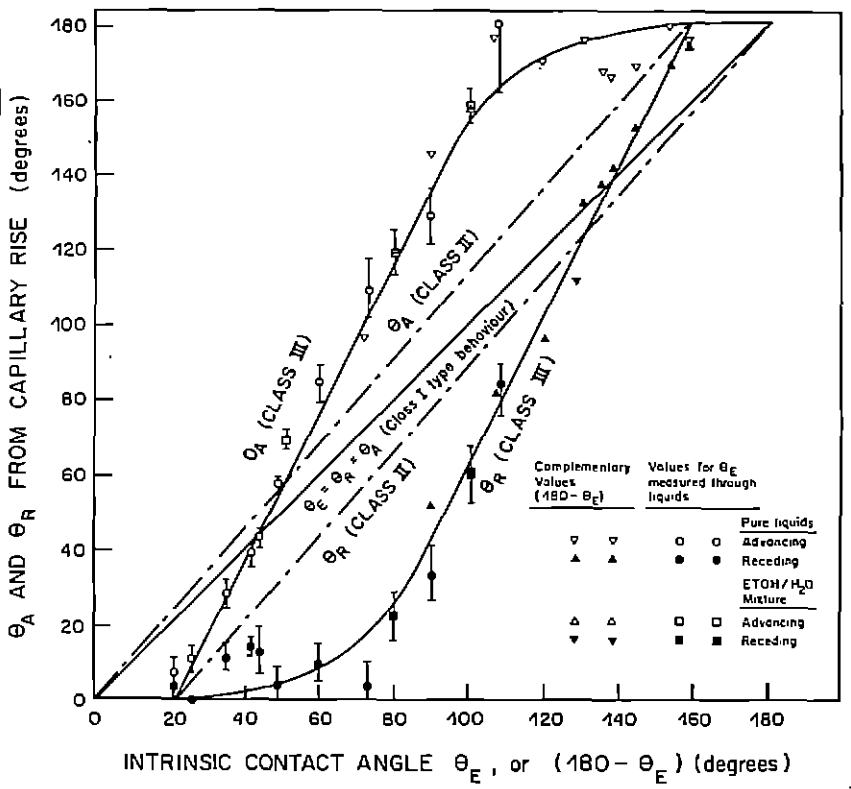
Model: allows modeling the hysteresis curves between advance/retreat angles from the intrinsic angles:
- Equal angles: advance/retreat angles identical to the intrinsic angle;
- Constant difference: constant difference between the advance/retreat angles and the intrinsic angle;
- Morrow curve: advance/retreat curves determined by Morrow curves;
 |
|---|
| Figure 10: Curves for each of the contact angle models implemented in GeoSlicer. Image taken from N. R. Morrow, 1975 (https://doi.org/10.2118/75-04-04). |
- Contact angle distribution center: Defines the center of the contact angle distribution;
- Contact angle distribution range: Distribution range (center-range/2, center+range/2), with the minimum/maximum angle being 0º/180º, respectively;
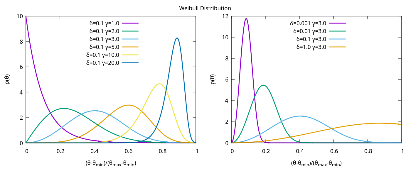
- Delta, Gamma: Truncated Weibull distribution parameters; if a negative number is chosen, a uniform distribution is used; If positive numbers are chosen, it uses the following probability distribution: \(p(\tilde\theta)=\frac{\gamma}{\delta}\frac{\tilde\theta^{\gamma-1}e^{-\tilde\theta^\gamma/\delta}}{1-e^{-1/\delta}}\) where \(\tilde\theta\in[\theta_{min},\theta_{max}]\). Some ideas for parameters for this distribution are graphed below:
 |
|---|
| Figure 11: Weibull distribution. |
- Contact angle correlation: Chooses how the contact angle will be correlated to the pore radius: Positive radius defines larger contact angles for larger radii; Negative radius does the opposite, assigning larger angles to smaller radii; Uncorrelated means independence between contact angles and pore radius;
- Separation: If the chosen model is constant difference, defines the separation between advance and retreat angles;
Other parameters are defined only for the second distribution:
- Fraction: A value between 0 and 1 that controls which fraction of the pores will use the second distribution instead of the first;
- Fraction distribution: Defines whether the fraction will be determined by the number of pores or total volume;
- Correlation diameter: If Fraction correlation is chosen as Spatially correlated, defines the most likely distance to find pores with the same contact angle distribution;
- Fraction correlation: Defines how the fraction for the second distribution will be correlated, if spatially correlated, for larger pores, smaller pores, or random;
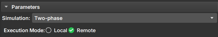
Execution Mode
The user can choose between two execution modes for running the two-phase simulation:
-
Local: Runs the simulation directly on the user’s machine.
In this mode, the user can define the Max subprocesses simulation option, which controls how many single-threaded subprocesses will run in parallel. The recommended value is about two-thirds of the total available CPU cores for optimal performance without overloading the system. -
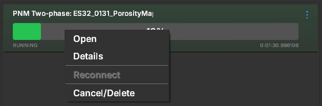
Remote: Sends the simulation to be executed on a configured computing cluster.
In this mode, the user specifies the Number of jobs into which the simulation will be divided. Ideal for very large sensitivity tests. The interface on the right will show the progress of the simulation, and the user can also Open the partial results for inspection before completion.
 |
|---|
| Figure 12a: Execution mode selection for the two-phase simulation. |
 |
|---|
| Figure 12b: Job options. |
This flexibility allows the user to take advantage of local processing for smaller test runs or to leverage cluster computing resources for more complex or large-scale simulations.
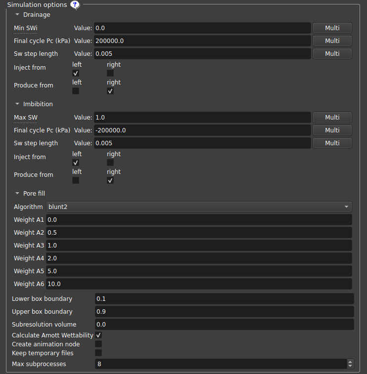
Simulation options
This section of parameters is dedicated to controlling the parameters related to the simulation itself.
 |
|---|
| Figure 13: Simulation parameters. |
- Minimum SWi: Sets the minimum SWi value, interrupting the drainage cycle when the Sw value is reached (SWi may be higher if water becomes trapped);
- Final cycle Pc: Interrupts the cycle when this capillary pressure is reached;
- Sw step length: Sw step used before checking the new permeability value;
- Inject/Produce from: Defines on which sides the fluid will be injected/produced along the z-axis; the same side can both inject and produce;
- Pore fill: Determines which mechanism dominates each individual pore filling event;
- Lower/Upper box boundary: Pores with a relative distance on the Z axis from the edge to this plane value are considered “left”/“right” pores, respectively;
- Subresolution volume: Considers that the volume contains this fraction of subresolution porous space that is always filled with water;
- Plot first injection cycle: If selected, the first cycle, oil injection into a fully water-saturated medium, will be included in the output graph. The simulation will run regardless of whether the option is selected or not;
- Create animation node: Creates an animation node that can be used in the “Cycles Visualization” tab;
- Keep temporary files: Keeps the .vtu files in the GeoSlicer temporary files folder, one file for each stage of the simulation;
- Max subprocesses: Maximum number of single-thread subprocesses to be executed; The recommended value for an idle machine is two-thirds of the total number of cores;
- Number of jobs: number jobs of into which the simulation will be divided on the cluster;
Since we have a vast number of parameters that can be modified to model the experiment from the simulation, it becomes useful to vary these parameters more systematically for an in-depth analysis of their influence on the results obtained.
To do this, the user can select the “Multi” button available in most parameters. When clicking on Multi, three boxes appear with start, end, and step options, which can be used to run several simulations in a linearly distributed table of the values of these parameters. If more than one parameter is chosen with multiple values, simulations run with all possible parameter combinations, which can considerably increase the number of simulations and the time to execute them.
Upon completion of the simulation set, the user can perform analyses to understand the relationships between the simulation results and the parameters selected in the Krel EDA tab.
Mercury injection
In addition to the one- and two-phase simulations, this module also offers a simulation of the Mercury intrusion experiment.
 |
|---|
| Figure 14: Mercury intrusion simulation. |
Mercury intrusion is an experiment in which liquid mercury is injected into a reservoir rock sample under vacuum, with increasing pressure. The volume of mercury invading the sample is measured as a function of mercury pressure. Since the contact angle of liquid mercury with mercury vapor is approximately independent of the substrate, analytical models, such as the tube bundle model, can be used to calculate the pore size distribution of the sample.
The mercury intrusion test is relatively affordable, and its main relevance in the context of PNM lies in the ability to perform the simulation on a sample for which experimental results of Mercury Intrusion Capillary Pressure (MICP) curves are available. This allows the comparison of results to validate and calibrate the pore network extracted from the sample, which will be used in one- and two-phase simulations.
To facilitate the analysis of sub-resolution pore radius assignment, the code in GeoSlicer will produce, in addition to the graphs obtained by the simulation in OpenPNM, graphs of pore and throat radius distributions and also volume distributions, separating them into resolved pores (which are not altered by subscale assignment) and unresolved pores. This allows the user to check whether the subscale model has been applied correctly.
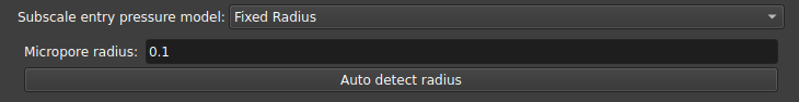
Subscale Model
In the case of a multiscale network, since the subscale radii cannot be determined from the image itself because they are outside the resolution, it is necessary to define a model for assigning these radii. Some options currently available are:
-
Fixed radius: All subresolution radii are the same size as chosen in the interface.
-
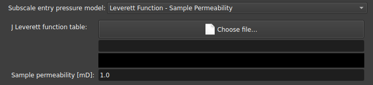
Leverett Function - Sample Permeability: Assigns an inlet pressure based on the J Leverett curve based on the permeability of the sample;
-
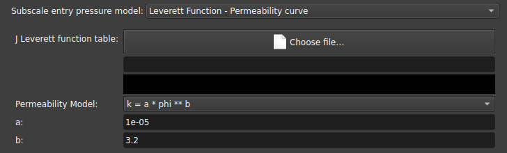
Leverett Function - Permeability curve: Also uses the J Leverett curve but with a curve defined for permeability instead of a value;
-
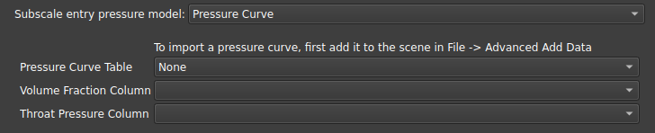
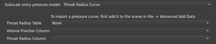
Pressure Curve and Throat Radius Curve: Assigns subresolution radii based on the curve obtained from a mercury injection experiment. The inlet pressure data can be used by volume fraction, or the equivalent radius can be used as a function of volume fraction;
Both models require a table containing the Incremental Pore Volume Fraction (\(\Delta S_i\)). This parameter represents the portion of the total pore space that is filled with mercury during a specific pressure interval (or, equivalently, the volume associated with a specific range of throat sizes). It is obtained from the experimental Mercury Intrusion Capillary Pressure (MICP) cumulative saturation (\(S_{Hg}\)) by calculating the difference between consecutive points: \(\Delta S_{i} = S_{Hg}(P_{i}) - S_{Hg}(P_{i-1})\). This fraction is used to weight the sub-resolution capillary functions, ensuring that the simulated mercury injection matches the experimental distribution of the sample.
The chosen subscale model has no impact on uniescalar network simulations, since all radii are already determined.
Kabs REV
The Pore Network Kabs REV module allows to perform single-phase (absolute permeability) simulations in multiple volume slices using the pore network.
It can be used to evaluate the quality in predicting the absolute permeability measurement, in order to discover what minimum volume size is needed to suppress the error due to finite size.
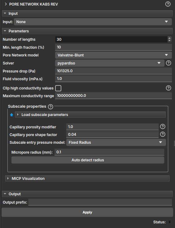
- Input: Expects as input a porosity map generated from the Microporosity module by segmentation. If the input is a porosity map, it will consider the multi-scale model. It is also allowed for the input to be a LabelMap generated through the Segment Inspector module, in which case a single-scale model will be considered, and the Subscale properties field can be ignored.
Parameters (Parameters)
- Number of lengths: number of length samples (or slices) to be considered in the simulation;
- Min. length fraction (%): minimum length fraction, in percentage, for defining the slices;
The other parameters are equivalent to those of the module that performs absolute permeability simulation. Read more in the PNM Simulation module.
Cycles Visualization
This module is used to control and visualize the relative permeability simulations created in the Pore Network Simulation module with the "Create animation node" option activated.
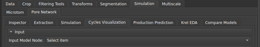 |
|---|
| Figure 1: Animation node input for visualization. |
Upon selecting the animation node, a model of the pores and connections will appear in the 3D visualization with arrows in the inlet/outlet regions, indicating the direction of invasions. Additionally, the graphs in the "Information" section will show the Krel curves and some extra information.
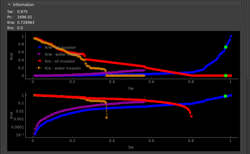 |
|---|
| Figure 3: Relative permeability curves for the cycle. |
From the parameters section in the interface, the user can then control the animation.
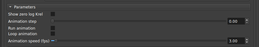 |
|---|
| Figure 3: Parameter selection interface. |
- Show zero log Krel: Sets a non-zero value for points on the logarithmic scale;
- Animations step: Selects a specific time step in the animation;
- Run animation: Incrementally updates the simulation step automatically;
- Loop animation: Executes the update in a loop, returning to the beginning whenever it reaches the end;
- Animation speed: Chooses the speed of the automatic update;
Krel EDA
EDA
To facilitate the analysis of the simulation set and understand how the different parameters affect the obtained results, the Krel EDA module was created.
After running several simulations using the Pore Network Simulation module, the user can input the table with the results obtained from that module, in order to visualize the curve cloud graphs, and also perform post-processing of their results.
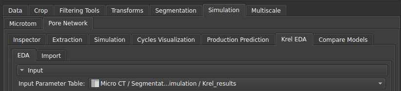 |
|---|
| Figure 1: Krel EDA module input. |
Various tools have been created to facilitate these analyses using interactive graphs.
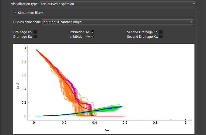
Krel curves dispersion
By selecting "Krel curves dispersion" as the visualization type, the dispersion graph of the krel curves from various simulations will be shown, along with their respective average.
It is possible to choose, using the selector boxes located just above the graph, which types of curves will be shown: drainage or imbibition curves and water and oil curves separately.
 |
|---|
| Figure 2: Krel curve cloud. |
To understand how these curves are distributed according to certain parameters, a color scale for the curves can be selected under "Curves color scale".
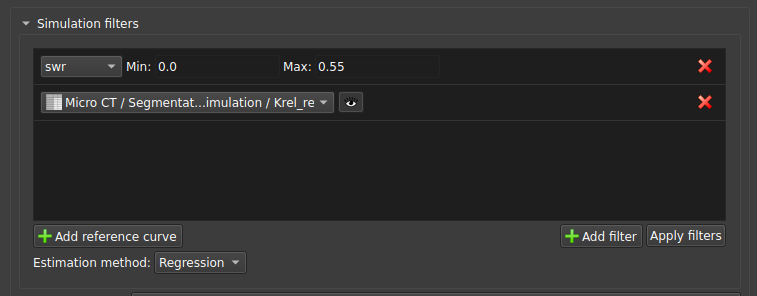
Filtering and adding reference curves
It is also possible to filter the curve cloud to show only a subset of the data using the collapsible section named "Simulation filters":
 |
|---|
| Figure 3: Filtered Krel curve cloud with a reference curve. |
There, it is possible to add a filter based on a parameter, and also add a reference curve, which could be experimental data, for example, for comparison.
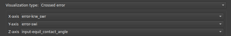
Crossed error
This visualization type is suitable for comparing the correlation between measurement errors and a parameter indicated by the color scale. The interface allows selecting which measurement error will be on the x and y axes, and also which parameter will be indicated on the color scale.
 |
|---|
| Figure 4: Crossed error visualization parameters. |
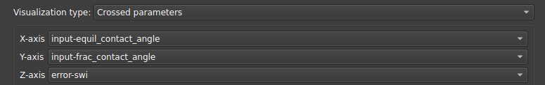
Crossed parameters
This visualization type serves to compare the correlation between parameters and the error indicated by the color scale. The interface allows selecting which parameter will be placed on the x and y axes, and also which error will be indicated on the color scale.
 |
|---|
| Figure 5: Crossed parameters visualization parameters. |
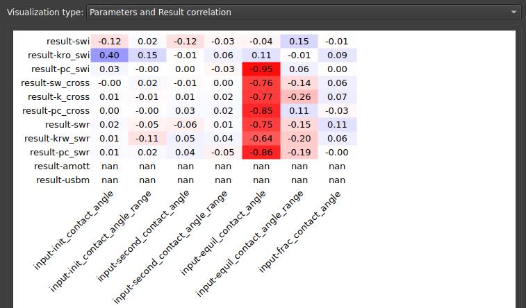
Parameters and Result correlation
In this visualization, the user can check the correlations between the simulation results and the parameters entered into the algorithm, thus identifying which parameters most affect the results.
 |
|---|
| Figure 6: Correlation between parameters and results. |
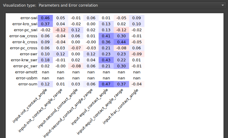
Parameters and Error correlation
Similarly, one might want to look at the correlations between simulation parameters and errors. This visualization type demonstrates this correlation matrix.
 |
|---|
| Figure 7: Correlation between parameters and errors. |
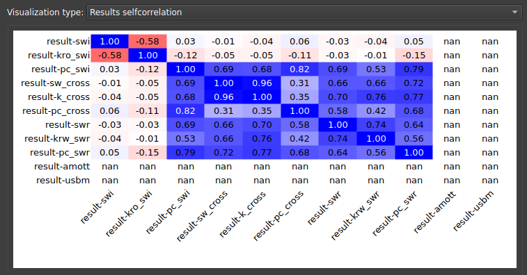
Results self-correlation
To understand how the results correlate with each other, i.e., how permeability is affected by saturation or pressure obtained in the simulation, one can look at the results' self-correlation matrix, presented in this visualization.
 |
|---|
| Figure 8: Results self-correlation matrix. |
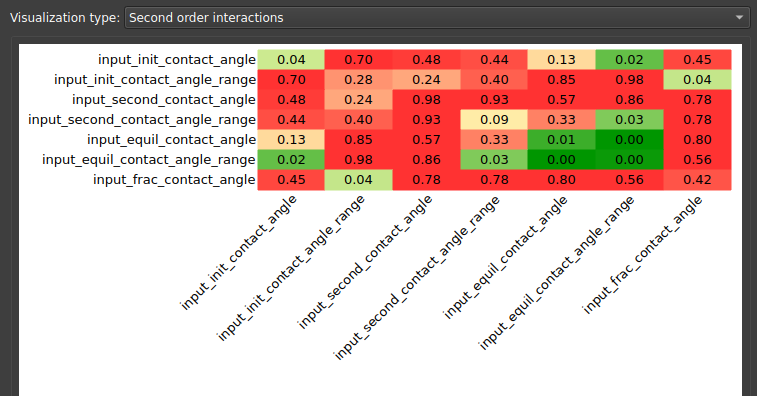
Higher order interactions
In statistical analysis, we might also want to understand the correlation reliability coefficients, which represent higher-order interactions than correlation. Three types of visualizations are available to interpret these higher-order dependencies: "Second order interactions", "Second order interactions list", "Third order interactions list".
 |
|---|
| Figure 9: Second-order interactions. |
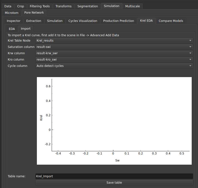
Import
The Import tab can be used to bring in results from an experimental table (for example) with krel curves. By selecting the columns corresponding to saturation, water permeability, oil permeability, and the cycle, the user can save a table to be used in the EDA module.
 |
|---|
| Figure 10: Import Tab. |
Production Prediction
This module can be used to estimate the amount of oil that can effectively be extracted for a given sample from the relative permeability curve, using the Buckley-Leverett equation.
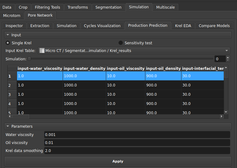
Single Krel
The first available option uses the relative permeability curve constructed for a single two-phase simulation.
 |
|---|
| Figure 1: Production module parameters. |
In the interface, in addition to the table with the simulation results, the user can choose the water and oil viscosity values that will be used in the estimation, as well as a smoothing factor for the krel curve.
 |
|---|
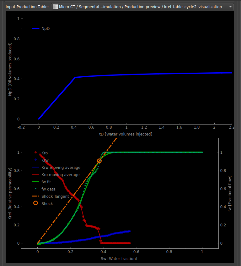
| Figure 2: Production estimation curve for single simulation. |
The generated graphs then correspond to the oil production estimation curve (in produced volume) based on the amount of water injected. And below, the relative permeability curve with an indication of the estimated shock wave.
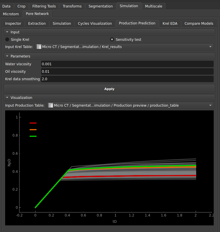
Sensitivity test
The other option can be used when multiple relative permeability curves are generated.
In this case, a cloud of curves will be generated and the algorithm also calculates the predictions: optimistic, pessimistic, and neutral.
 |
|---|
| Figure 3: Production estimation curve for the sensitivity test. |
Fluxos
Absolute Permeability Simulation (Kabs)
Single-scale Kabs Simulation
The workflow below allows simulating and obtaining an estimate of absolute permeability in a single-scale sample, considering all pores as resolved:
- Load the volume in which you want to run the simulation;
- Perform Manual Segmentation using one of the segments to designate the porous region of the rock;
- Separate the segments using the Inspector tab, thus delimiting the region of each pore;
- Use the Extraction tab to obtain the pore and throat network from the generated LabelMap volume;
- On the Simulation tab to run the Kabs simulation;
Relative Permeability (Krel) Simulation
Single Krel Simulation (animation)
The workflow below allows you to simulate and obtain an animation of Drainage and Imbibition processes:
- Load the volume on which you want to run the simulation;
- Perform Manual Segmentation using one of the segments to designate the porous region of the rock;
- Separate the segments using the Inspector tab, thus delineating the region of each pore;
- Use the Extraction tab to obtain the pore and throat network from the generated LabelMap volume;
- On the Simulation tab;
- Check the option "Create animation node" in the "Simulation options" box and click the "Apply" button;
- Upon finishing the simulation, go to the "Cycles Visualization" tab and select the animation node to visualize the generated cycle and curve;
Sensitivity Test
The workflow below allows the user to simulate and obtain a cloud of Krel curves from which they can perform different analyses to determine the most sensitive properties:
- Load the volume on which you want to run the simulation;
- Perform Manual Segmentation using one of the segments to designate the porous region of the rock;
- Separate the segments using the Inspector tab, thus delineating the region of each pore;
- Use the Extraction tab to obtain the pore and throat network from the generated LabelMap volume;
- On the Simulation tab, choose the pore table, in the Simulation selector select "Two-phase";
- Select multiple values for some parameters by clicking the "Multi" button (as we did for the center of the contact angle distributions in the video) - You can find more information about the parameters in the "Two-phase" section;
- (Optional) Save the selected parameters using the "Save parameters" section;
- Click the "Apply" button to run the various simulations;
- Upon finishing the execution, go to the "Krel EDA" tab and select the generated parameters table to perform different analyses using the interface's visualization features (curve cloud, parameter and results correlations, etc.);
Production Estimation
The workflow below allows the user to simulate and obtain a cloud of Krel curves, on a single-scale sample:
- Load the volume on which you want to run the simulation;
- Perform Manual Segmentation using one of the segments to designate the porous region of the rock;
- Separate the segments using the Inspector tab, thus delineating the region of each pore;
- Use the Extraction tab to obtain the pore and throat network from the generated LabelMap volume;
- Select multiple values for some parameters by clicking the "Multi" button (as we did for the center of the contact angle distributions in the video) - You can find more information about the parameters in the "Two-phase" section;
- (Optional) Save the selected parameters using the "Save parameters" section;
- Click the "Apply" button to run the various simulations;
- Upon finishing the execution, go to the "Production Prediction" tab and select the parameters table generated in the simulation; Two options are available in this interface:
- The first one, "Single Krel," is an analysis of each individual simulation;
- The second, "Sensitivity test," is a production estimation considering all simulations performed;
Mercury Intrusion Simulation
MICP Simulation
The workflow below allows simulating the Mercury Intrusion experiment on the sample:
- Load the volume in which you want to run the simulation;
- Perform Manual Segmentation using one of the segments to designate the porous region of the rock;
- Separate the segments using the Inspector tab, thus delimiting the region of each pore;
- Use the Extraction tab to obtain the pore and throat network from the generated LabelMap volume;
- In the Simulation tab, choose the pore table, in the Simulation selector select Mercury injection;
- Upon completion of the simulation, the results can be viewed in the generated table or in the created graphs;
Report Generation
The workflow below allows running a complete PNM workflow, performing Kabs, Krel, and MICP simulations; The results can be viewed in a web interface:
- Load the volume on which you want to execute the simulation;
- Perform Manual Segmentation using one of the segments to designate the porous region of the rock;
- Separate the segments using the Inspector tab, thus delimiting the region of each of the pores;
- Use the Microtom tab and select "PNM Complete Workflow";
- Select or create a parameter selection table for the "Teste de Sensibilidade" by clicking the "Edit" button;
- Click on "Apply" to run the workflow;
- After the simulation is complete, click the "Open Report Locally" button to open the report.