Note
Some features presented on this page will only be available in the private version of GeoSlicer. Learn more by clicking here.
ImageLog Import
GeoSlicer module for loading profile data in DLIS, LAS, and CSV, as described in the steps below:
-
Select the well log file under Well Log File.
-
Edit Null values list and add or remove values from the list of possible null values.
-
Choose the desired profiles to be loaded into GeoSlicer, according to each option described below:
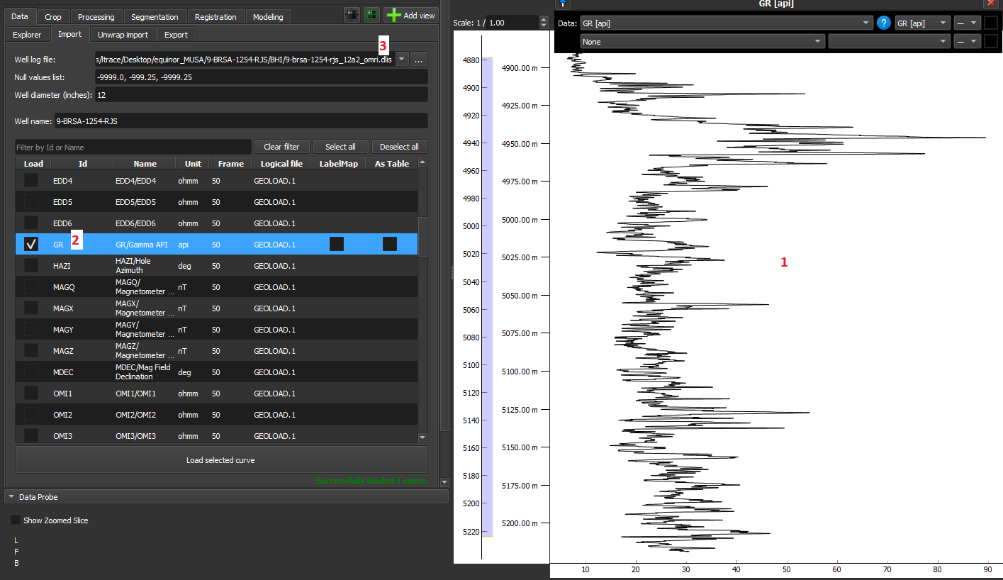
- 1-D data should be loaded without selecting the “As Table“ and “LabelMap” options and are displayed as line graphs in the Image Log View.
-
2-D data can be loaded as volumes, tables, or LabelMap in GeoSlicer, with each of the options detailed below:
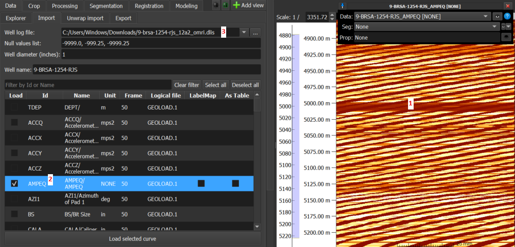
- Volume: This is the default GeoSlicer option, without checking 'As Table' and 'LabelMap', where the data is loaded as a volume and displayed as an image in the Image Log View.
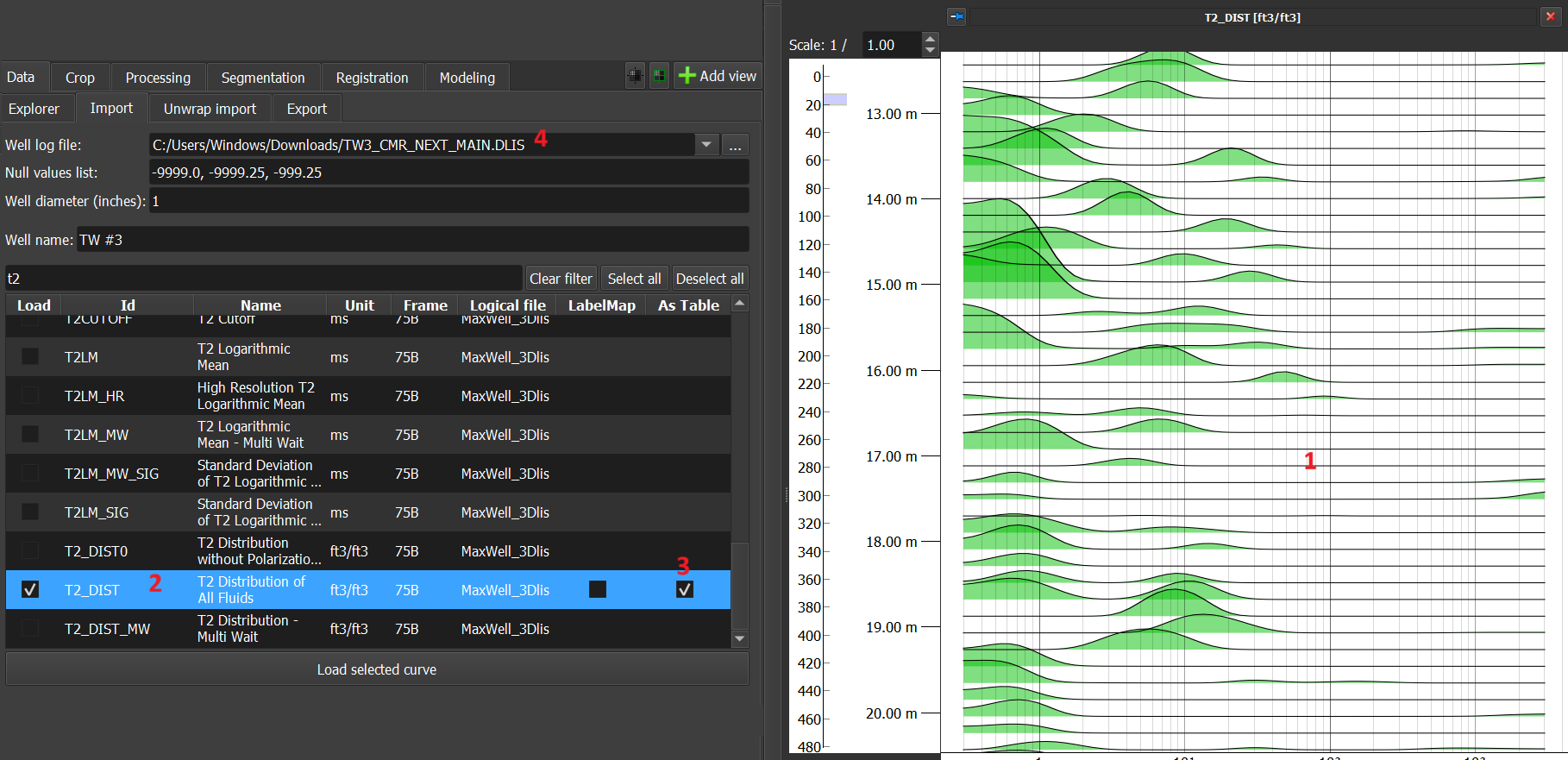
- Tables: In this option, by checking the 'As Table' checkbox, the data is loaded as a table and is displayed as several histograms, as in the case of the t2_dist data in Figure 3 below:
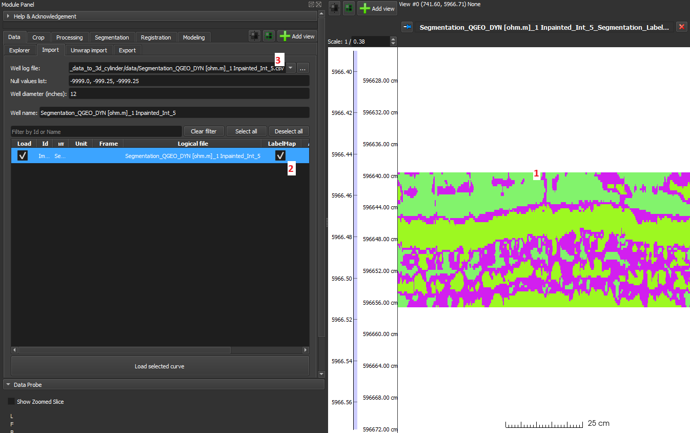
- LabelMap: In this option, by checking the 'LabelMap' checkbox, assuming segmented data, it is loaded as a LabelMap and displayed as a segmented image.
- Volume: This is the default GeoSlicer option, without checking 'As Table' and 'LabelMap', where the data is loaded as a volume and displayed as an image in the Image Log View.
- 1-D data should be loaded without selecting the “As Table“ and “LabelMap” options and are displayed as line graphs in the Image Log View.
Formatting of files to be loaded
LAS
Sequential curves with mnemonics in the format mnemonic[number] will be grouped into 2-D data. For example, the mnemonics of an image with 200 columns:
AMP[0]
…
AMP[199]
The same file can contain both 1-D and 2-D data. In the following example, AMP is an image, while LMF1 and LMF2 are 1-D data:
AMP[0]
…
AMP[199]
LMF1
LMF2
CSV
For GeoSlicer to interpret CSV data as 2-D, the mnemonics simply need to be of the same name followed by an index in square brackets, as in the 1st example of the LAS section above (AMP[0], …, AMP[199]). Unlike the LAS case, the file must contain only 2-D data.
Unwrapped Tomographic Image Importer (Unwrap)
The Unwrapped Tomographic Image Importer module is a specialized tool for loading and reconstructing image profiles from 2D drill core images that have been scanned and "unwrapped".
In some workflows, the borehole wall image is obtained by scanning drill cores and then unwrapping this cylindrical image into a 2D representation. This module serves to import these 2D images (in formats such as JPG, PNG, or TIF) and reconstruct them into a profile image with the correct depth in GeoSlicer. It uses a CSV file to obtain depth information and a well diameter to correctly scale the image's circumference.
Input Requirements
To use this importer, your files must follow strict naming and structural conventions.
Image File Naming Convention
Image files must be named following the pattern:
T<ID_testemunho>_CX<primeira_caixa>CX<ultima_caixa>.<extensao>
T<ID_testemunho>: The numeric identifier of the core._CX<primeira_caixa>CX<ultima_caixa>: The range of core boxes contained in the image file.<extensao>: The file extension (e.g.,jpg,png,tif).
Example: T42_CX1CX5.jpg refers to core 42 and contains images from boxes 1 to 5.
Boundaries File (CSV)
A CSV file is required that maps each core box to its top and base depths. The file must contain the following columns:
poco: The well name.testemunho: The core ID (must match the one used in the file name).caixa: The box number.topo_caixa_m: The top depth of the box in meters.base_caixa_m: The base depth of the box in meters.
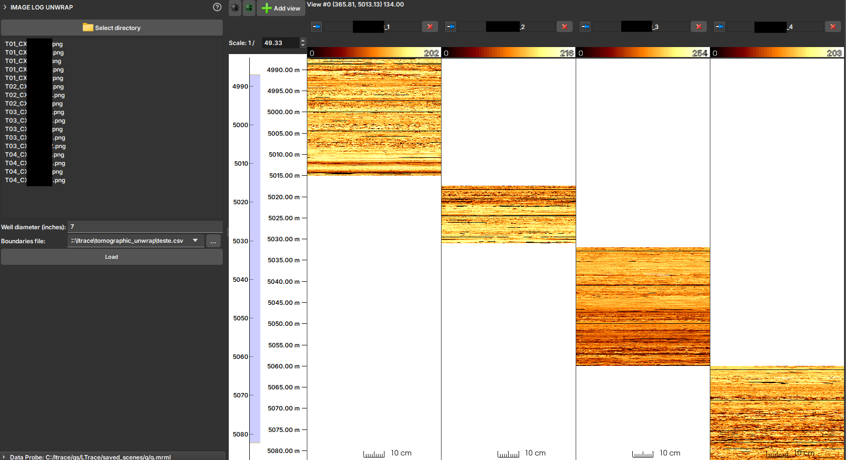
How to Use
- Select directory: Click the button to choose the folder containing the unwrapped image files and the boundaries CSV file.
- Check Files: The list of detected image files will be displayed. The module will attempt to automatically find and select a
.csvfile in the same directory. - Well diameter (inches): Enter the well diameter in inches. This value is crucial for correctly scaling the image width to the well's circumference.
- Boundaries file: If the CSV file is not automatically selected, point to the correct location in this field.
- Load: Click the button to start the import.
Output
The module will process the images and create one or more profile images in the scene. Each image represents a complete core, assembled from its respective image files and positioned at the correct depths. The generated images will be organized in a folder with the same name as the input directory within the project hierarchy.
MicroCT Import
The micro CT environment has only one Loader to load 3D volumes. It is capable of recognizing various types of data, such as:
- RAW: Image files in RAW format.
- TIFF: Image files in TIFF format.
- PNG: Image files in PNG format.
- JPG: Image files in JPG format.
With the exception of the RAW format, the Loader requires a directory containing the 2D images that make up the volume. The Loader will recognize the images and assemble the volume automatically. Below we will detail these two modes of operation.
Viewing TIFF, PNG, and JPG formats
- Click the Choose folder button to select the directory containing micro CT images. In this option, the directory needs to contain 2D images to compose the 3D volume.
- Upon selecting the directory, the module reports how many images it found, so that the user can confirm that all images were detected correctly. If images are missing, the user can check if the name of any of them is not outside the standard, causing the detection failure.
- Automatically, the module attempts to detect the pixel size of the images through the file name (e.g., prefix "_ 28000nm). If the detected value is not correct, the user can change the value manually.
- Click the Load micro CTs button to load the images. The 3D volume will be assembled and made available in the main View and accessible via Explorer.
Viewing RAW format
- Click the Choose file button to select the RAW file.
- As the .RAW file does not contain image information directly in the format, the module attempts to infer the data settings from the file name. For example, AFLORAMENTO_III_LIMPA_B1_BIN_1000_1000_1000_02214nm.raw
- Pixel size: 2214nm
- Volume size: 1000x1000x1000
- Pixel type: BIN (8 bit unsigned)
- The user can manually change the volume settings, such as pixel size, volume size, and data type, if any information was not detected correctly or simply does not exist.
- Click the Load button to load the volume. The 3D volume will be assembled and made available in the main View and accessible via Explorer.
Exploring Import Parameters
There is a Real-time update option that allows the volume to be updated automatically as settings are changed. However, we recommend that the user does not use this option for very large volumes.
- Change the X dimension field until straight columns appear in the image (if the columns are slightly inclined then the value is close to being correct). Try with different endianness and pixel type values if no value in X dimension seems to make sense.
- Move Header size until the first row of the image appears at the top.
- Change the value of the Z dimension field to a few tens of slices to make it easier to see when the Y dimension value is correct.
- Change the value of Y dimension until the last row of the image appears at the bottom.
- Change the Z dimension slider until all image slices are included.
Advanced Import Features
Auto-crop
The user can enable the Auto-crop Rock Cylinder option to automatically crop the image. This solution is applied to cases where the study volume is a cylinder, typically surrounded by other layers of different materials. This option attempts to detect the relevant cylinder and generate a region to crop. Before applying the crop, the module presents the detected region so that the user can confirm if the region is correct or make adjustments to frame the region of interest.
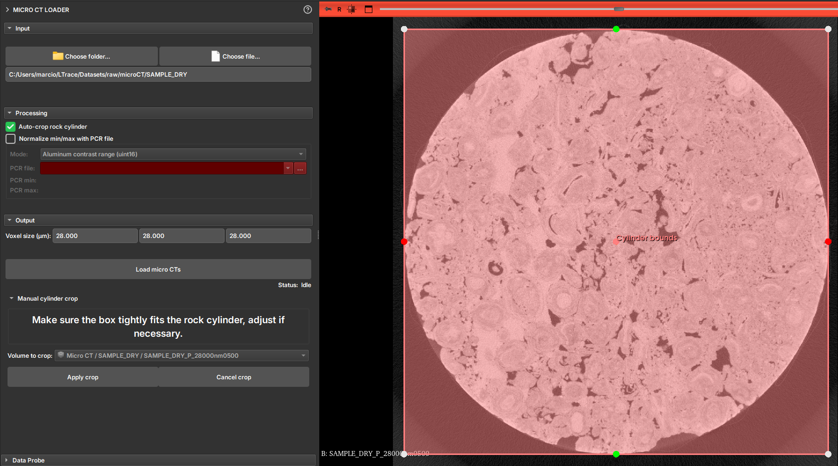
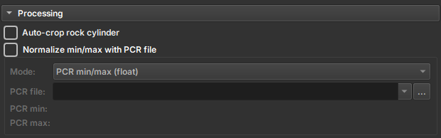
Image Normalization
Some images can be imported using a value normalization file, the PCR. To do this, the user must select the Normalize min/max with PCR file option and select the corresponding PCR file. The file usage options are:
- Normalize min/max (float): Normalizes the image values based on the PCR file.
- Divide by alumminum median (float): Divides the image values by the aluminum median.
- Alumminum contrast range (uint8): Defines the aluminum contrast range.
Multicore
GeoSlicer module for processing, orienting, and unwrapping cores in batches. A demonstration video of an earlier version of GeoSlicer is available.
Panels and their usage
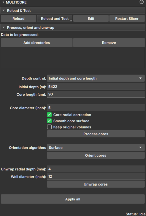 |
|---|
| Figure 1: Multicore Module. |
Data selection
-
Add directories: Adds directories containing core data. These directories will appear in the Data to be processed list. During execution, data search will occur only one level down.
-
Remove: Removes directories from the search list.
-
Depth control: Choose the method to configure core boundaries:
- Initial depth and core length:
- Initial depth (m): Depth of the top of the core.
- Core length (cm): Length of the core.
- Core boundaries CSV file:
- Core depth file: Selector for a CSV file containing core boundaries in meters. The file must have two columns, with each row corresponding to a different core, in processing order. The columns should indicate, respectively, the upper and lower depth boundaries.
- Initial depth and core length:
-
Core diameter (inch): Approximate core diameter in millimeters.
Processing
Check the option you wish to execute:
-
Core radial correction: Corrects attenuation effects of core CT, such as beam hardening. Applies a correction factor to all image slices (transverse images, xy plane) to standardize attenuation in terms of radial coordinates. The correction factor is calculated based on the average of all slices and depends only on the radial distance from the center of the slices.
-
Smooth core surface: Applies smoothing (anti-aliasing) to the core surface.
-
Keep original volumes: Saves the original data without corrections and without smoothing.
-
Process cores: Processes the cores in the directories in the order they were added. Once loaded, the data can be viewed in the Explorer module.
Orientation
-
Orientation algorithm: Choose a core orientation algorithm:
-
Surface: Orientation is based on the longitudinal cutting angle of the core ends. This option is better in cases where the cutting angle is not shallow and if the ends are well preserved (cleaner cutting surfaces).
-
Sinusoid: Uses core unwrapping to find the sinusoidal patterns created by depositional layers to orient the cores. This option is good if the depositional layers are well pronounced in the core group.
-
Surface + Sinusoid: If the Surface algorithm is able to find an alignment, it will be used; otherwise, the Sinusoid algorithm will be applied instead.
-
-
Orient cores: Applies rotation along the longitudinal axis of the core, according to the selected algorithm. The first core determines the orientation of subsequent ones.
Unwrap
-
Unwrap radial depth (mm): Enter a value ranging from 0 up to the core radius, in millimeters. From the outside of the core to the center, along the radial axis, this is the depth at which the unwrap will be generated. Use small values if you want to unwrap close to the core surface.
-
Well diameter: Enter the approximate well diameter (greater than the core diameter) which will be used to project the core image onto the well wall.
-
Unwrap cores: Generates the unwrapped images of the core and the well. The images preserve the core scale along all axes. Thus, pixel size and upscaling do not depend on the core radius. The delta angle used in the iterative process of collecting unwrapped voxels is defined as pixel_size/radius.
Apply all
Applies all processing, orientation, and unwrapping steps.
Common Problems
"Could not detect core geometry"
The error "Could not detect core geometry" occurs in the Multicore module when the CoreGeometryCLI command-line interface fails to detect any valid core geometry in the provided volume. This happens because the CLI is unable to find circular features (representing the core) in the volume slices using image processing techniques.
Primary reasons this error can occur:
1. No Detectable Core Circles in the Volume
- The volume image does not contain a clear, cylindrical core structure that can be identified via Hough circle detection.
- Possible causes:
- The core is obscured, damaged, or has irregular geometry that doesn't form detectable circles in cross-sections.
- Low image quality, noise, or artifacts prevent edge detection from working properly.
2. Incorrect Core Radius Parameter
- The
coreRadiusvalue passed to the CLI is inaccurate, causing the search radius range (min/max) to not match the actual core size in the image. - The search radius is calculated as
[coreRadius - 3mm, coreRadius + 3mm]in pixels. If the real core radius is outside this range, no circles will be detected. - Users should verify the core radius matches the physical dimensions of the sample by loading the original volume and measuring the radius.
3. Insufficient Valid Slices for Analysis
- The CLI discards 20 slices from each end of the volume to avoid "destroyed core ends," then samples every 5th slice.
- If the volume has very few slices (e.g., <40 total), there may be no slices left to analyze after discarding ends.
- If all sampled slices fail the geometry detection (e.g., due to poor image quality in those slices), the result list remains empty.
4. Circle Detection Filtering
- Detected circles are filtered out if their center is too close to the image center (within 10% of the minimum image dimension from the center). This is to avoid false positives from central artifacts.
- If all detected circles are filtered out by this condition, no valid geometry is recorded.
Troubleshooting Steps for Users
- Verify Input Data: Ensure the volume is a valid core image with clear circular cross-sections. Check volume dimensions and spacing.
- Adjust Core Radius: Provide an accurate core radius in meters. If unsure, try a range of values.
- Check Volume Quality: Load only the original core image to confirm the core is visible and not obscured.
If the error persists, the volume may not be suitable for automated core geometry detection, and manual intervention or alternative modules might be needed.