More Tools
Volume Calculator
The Volume Calculator module performs mathematical and logical operations using the volumes loaded in the project. It is a flexible tool for combining, modifying, and analyzing volumetric data through custom formulas.
Step 1: Write the Formula
- Locate the volumes you want to use. You can use the filter field to find them more easily.
- In the Formula field, type the desired mathematical expression.
- To insert a volume into the formula, type its name exactly as it appears in the data tree, enclosing it in curly braces
{}. Alternatively, double-click on the volume name in the data tree to have it automatically inserted into the Formula field.
Here are some examples of valid formulas:
-
Simple arithmetic operation:
This formula adds the values of{Volume1} + log({Volume2})Volume1with the logarithm of the values ofVolume2. -
Mask creation (thresholding):
This formula generates a new binary volume (mask). Regions where{Volume1} < 10000Volume1values are less than 10000 will receive the value 1, and the others will receive the value 0. -
Mask application:
This formula first creates a mask for({Volume1} > 13000) * {Volume1}Volume1values greater than 13000 and then multiplies this mask by the originalVolume1. The result is a volume where values below the threshold are zeroed out.
Complete list of available operators and functions
Step 2 (Optional): Use Mnemonics
If volume names are too long or complex, you can use mnemonics (aliases) to simplify writing the formula.
- Expand the Mnemonics section.
- Click on the Mnemonic Table selector to choose an existing table or create a new one.
- If you create a new table, it will appear in the preview area. Double-click on the cells to edit and associate a Volume name with a Mnemonic.
- Use the Add mnemonic and Remove selected mnemonics buttons to add or remove rows from the table.
- With a mnemonic table selected, when you double-click on a volume in the data tree, its mnemonic will be inserted into the formula instead of its full name.
Note
Mnemonic tables are saved in the GeoSlicer scene within a folder called Volume Calculator Mnemonics, allowing them to be reused in future calculations.
Step 3: Define the Output Volume
- In the Output volume name field, type the name for the new volume that will be generated with the calculation result.
Step 4: Execute the Calculation
- Click the Calculate button.
- The operation will be executed, and a status bar will show the progress.
- At the end, the new output volume will be added to the scene, usually in the same folder or directory as the first volume used in the formula.
Geometry Alignment (Resampling)
If the volumes used in the formula have different geometries (distinct dimensions, spacing, or origin), all volumes will be automatically resampled temporarily to match the geometry of the first volume listed in the formula. Although this resampling is necessary for the calculation, it can introduce interpolation into the data. Verify that the order of the volumes in the formula is in accordance with the expected result.
Table Filter
This module filters tables of element properties (such as pores or grains) that have been individualized by segmentation algorithms. For more details on the origin of this data, consult the Segment Inspector documentation.
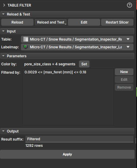
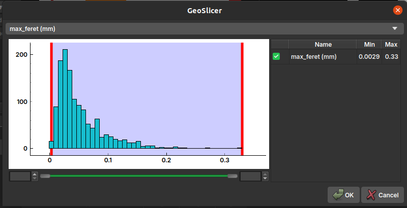
In the module's interface, the user can select the input table and build specific filters for each of its columns. A central feature of this module is instant visual feedback: as filters are applied, the corresponding elements in the LabelMap are updated in real-time, allowing for visual and interactive analysis.
It is possible to add multiple rules to create a complex filter, and the user can choose to keep or remove the rows that meet the established criteria.
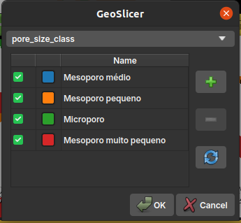
It is also possible to assign a different color to each pore class, facilitating visualization and analysis. By default, the color is associated with the pore_size_class classification.
Properties Description
- label: A unique index for each of the individualized elements;
- voxelCount: The number of voxels that make up each element;
- volume (mm³): The actual volume of the element, calculated from the
voxelCountand the image's voxel size; - max_feret (mm): The maximum Feret diameter, which represents the greatest distance between two parallel points on the element's boundary. It is a measure of the element's maximum size;
- aspect_ratio: The aspect ratio, usually calculated as the ratio between the largest and smallest axis of the element. A value close to 1 indicates that the element is approximately isometric (like a sphere or cube), while larger values indicate a more elongated shape;
- elongation: Measures how elongated an object is. It is the square root of the ratio between the second and first moment of inertia of the object. A value of 0 corresponds to a circle or sphere, and larger values indicate greater elongation;
- flatness: Measures how flat an object is. It is the square root of the ratio between the third and second moment of inertia of the object. A value of 0 corresponds to a circle or sphere, and larger values indicate greater flatness.;
- ellipsoid_area (mm²): The surface area of an ellipsoid that has the same moments of inertia as the element;
- ellipsoid_volume (mm³): The volume of an ellipsoid that has the same moments of inertia as the element.
- ellipsoid_area_over_ellipsoid_volume (1/mm): The ratio between the surface area and the volume of the equivalent ellipsoid. This measure is useful for characterizing the element's surface-to-volume ratio;
- sphere_diameter_from_volume (mm): The diameter of a sphere that has the same volume as the element. It is a way to estimate an "equivalent" diameter for irregular shapes;
- pore_size_class: A categorical classification of pore size (e.g., micropore, mesopore, macropore) based on one of the size measurements;
Tables
This module is used to manipulate and edit tables within GeoSlicer.
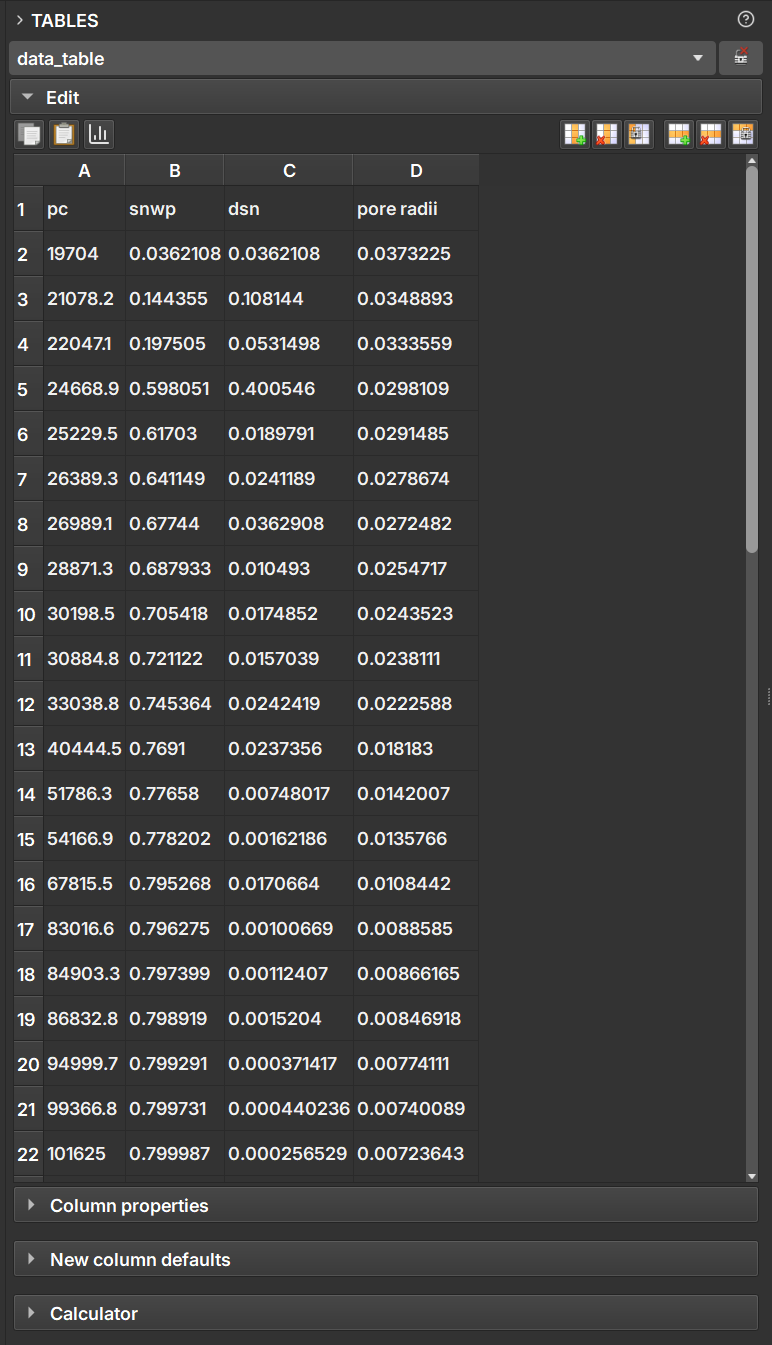
By selecting a table node, the user can edit each of the cells as in a spreadsheet application. From the buttons located above the table, it is also possible to include/remove rows and columns, as well as make copies.
In the Column properties field, you can convert between the data types presented in the table columns.
In the Calculator field, the user can perform simple mathematical operations between the columns to generate new data columns.
Charts
This module is used to generate charts based on a table node generated in GeoSlicer. In the module interface, the user can select one or more tables to generate a chart based on the data.
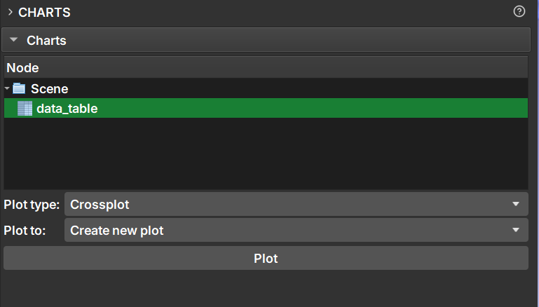
After selecting the tables with the data to be plotted, you can select the chart type in the Plot type field; the chart options are:
- Crossplot: A combination of a scatter plot, with histograms for each of the axes and color selection according to a third column.
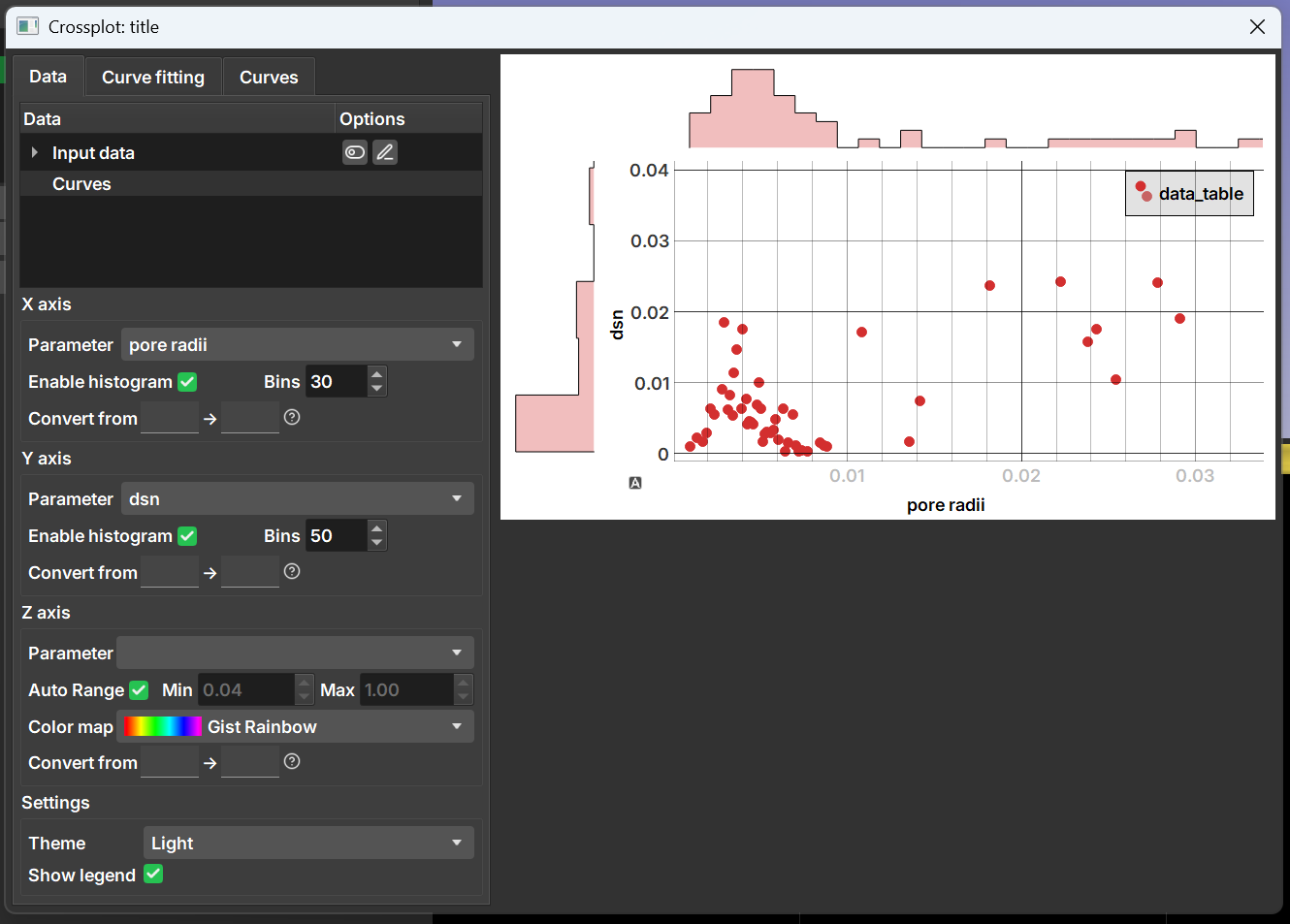
Allows curve fitting or addition of curves to the chart for comparison in the "Curve fitting" and "Curves" tabs.
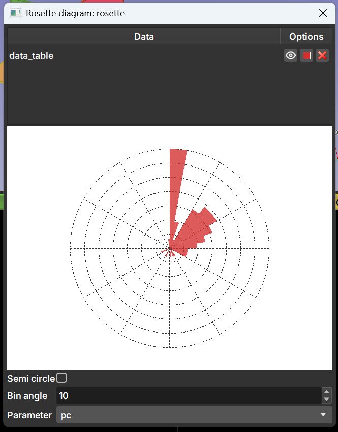
- Rosette Diagram: Diagram typically used to show the frequency and distribution of directional data.
-
Transition
-
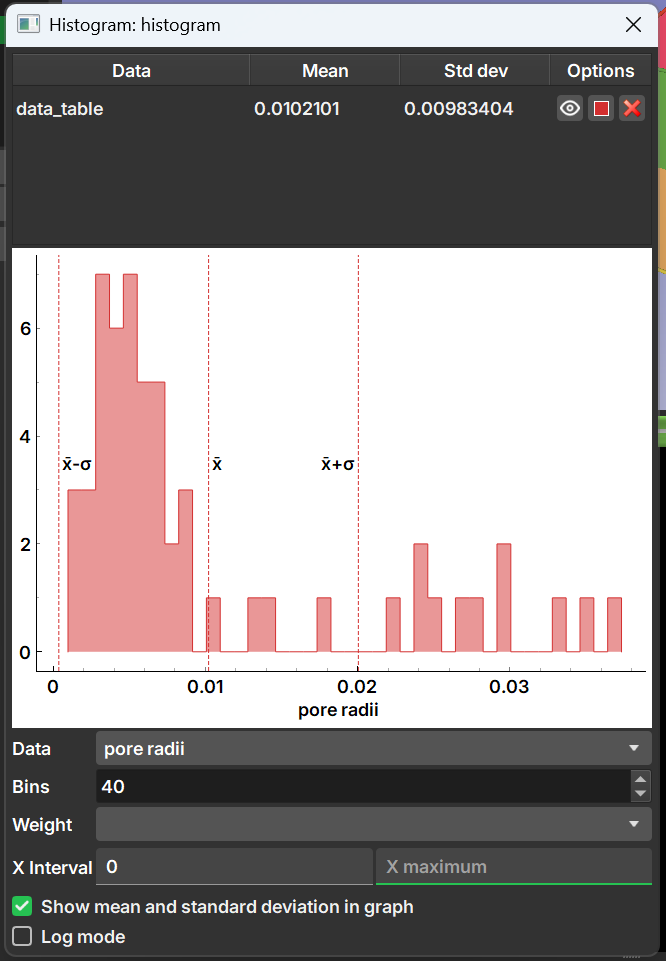
Histograms in depth
-
Histogram: Simple histogram of the data in one of the columns. Allows selection of the number of bins and re-weighting according to another column.