More Tools
Volume Calculator
The Volume Calculator module performs mathematical and logical operations using the volumes loaded in the project. It is a flexible tool for combining, modifying, and analyzing volumetric data through custom formulas.
Step 1: Write the Formula
- Locate the volumes you want to use. You can use the filter field to find them more easily.
- In the Formula field, type the desired mathematical expression.
- To insert a volume into the formula, type its name exactly as it appears in the data tree, enclosing it in curly braces
{}. Alternatively, double-click on the volume name in the data tree to have it automatically inserted into the Formula field.
Here are some examples of valid formulas:
-
Simple arithmetic operation:
This formula adds the values of{Volume1} + log({Volume2})Volume1with the logarithm of the values ofVolume2. -
Mask creation (thresholding):
This formula generates a new binary volume (mask). Regions where{Volume1} < 10000Volume1values are less than 10000 will receive the value 1, and the others will receive the value 0. -
Mask application:
This formula first creates a mask for({Volume1} > 13000) * {Volume1}Volume1values greater than 13000 and then multiplies this mask by the originalVolume1. The result is a volume where values below the threshold are zeroed out.
Complete list of available operators and functions
Step 2 (Optional): Use Mnemonics
If volume names are too long or complex, you can use mnemonics (aliases) to simplify writing the formula.
- Expand the Mnemonics section.
- Click on the Mnemonic Table selector to choose an existing table or create a new one.
- If you create a new table, it will appear in the preview area. Double-click on the cells to edit and associate a Volume name with a Mnemonic.
- Use the Add mnemonic and Remove selected mnemonics buttons to add or remove rows from the table.
- With a mnemonic table selected, when you double-click on a volume in the data tree, its mnemonic will be inserted into the formula instead of its full name.
Note
Mnemonic tables are saved in the GeoSlicer scene within a folder called Volume Calculator Mnemonics, allowing them to be reused in future calculations.
Step 3: Define the Output Volume
- In the Output volume name field, type the name for the new volume that will be generated with the calculation result.
Step 4: Execute the Calculation
- Click the Calculate button.
- The operation will be executed, and a status bar will show the progress.
- At the end, the new output volume will be added to the scene, usually in the same folder or directory as the first volume used in the formula.
Geometry Alignment (Resampling)
If the volumes used in the formula have different geometries (distinct dimensions, spacing, or origin), all volumes will be automatically resampled temporarily to match the geometry of the first volume listed in the formula. Although this resampling is necessary for the calculation, it can introduce interpolation into the data. Verify that the order of the volumes in the formula is in accordance with the expected result.
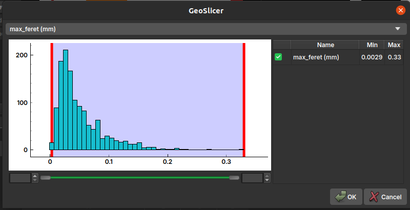
Table Filter
This module filters tables of element properties (such as pores or grains) that have been individualized by segmentation algorithms. For more details on the origin of this data, consult the Segment Inspector documentation.
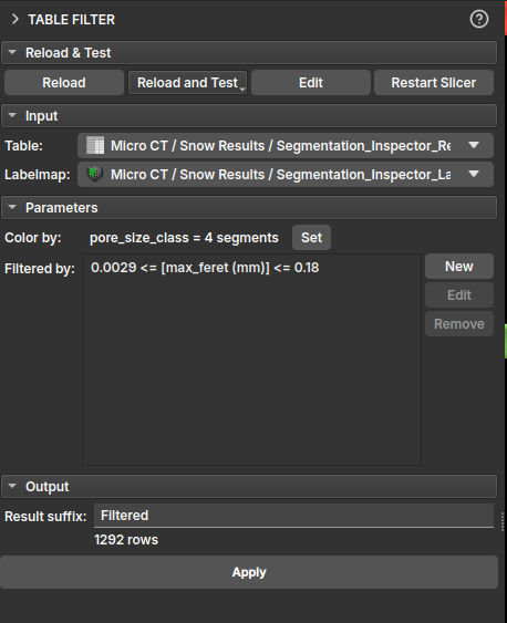
In the module's interface, the user can select the input table and build specific filters for each of its columns. A central feature of this module is instant visual feedback: as filters are applied, the corresponding elements in the LabelMap are updated in real-time, allowing for visual and interactive analysis.
It is possible to add multiple rules to create a complex filter, and the user can choose to keep or remove the rows that meet the established criteria.
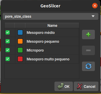
It is also possible to assign a different color to each pore class, facilitating visualization and analysis. By default, the color is associated with the pore_size_class classification.
Properties Description
- label: A unique index for each of the individualized elements;
- voxelCount: The number of voxels that make up each element;
- volume (mm³): The actual volume of the element, calculated from the
voxelCountand the image's voxel size; - max_feret (mm): The maximum Feret diameter, which represents the greatest distance between two parallel points on the element's boundary. It is a measure of the element's maximum size;
- aspect_ratio: The aspect ratio, usually calculated as the ratio between the largest and smallest axis of the element. A value close to 1 indicates that the element is approximately isometric (like a sphere or cube), while larger values indicate a more elongated shape;
- elongation: Measures how elongated an object is. It is the square root of the ratio between the second and first moment of inertia of the object. A value of 0 corresponds to a circle or sphere, and larger values indicate greater elongation;
- flatness: Measures how flat an object is. It is the square root of the ratio between the third and second moment of inertia of the object. A value of 0 corresponds to a circle or sphere, and larger values indicate greater flatness.;
- ellipsoid_area (mm²): The surface area of an ellipsoid that has the same moments of inertia as the element;
- ellipsoid_volume (mm³): The volume of an ellipsoid that has the same moments of inertia as the element.
- ellipsoid_area_over_ellipsoid_volume (1/mm): The ratio between the surface area and the volume of the equivalent ellipsoid. This measure is useful for characterizing the element's surface-to-volume ratio;
- sphere_diameter_from_volume (mm): The diameter of a sphere that has the same volume as the element. It is a way to estimate an "equivalent" diameter for irregular shapes;
- pore_size_class: A categorical classification of pore size (e.g., micropore, mesopore, macropore) based on one of the size measurements;
Tables
This module is used to manipulate and edit tables within GeoSlicer.
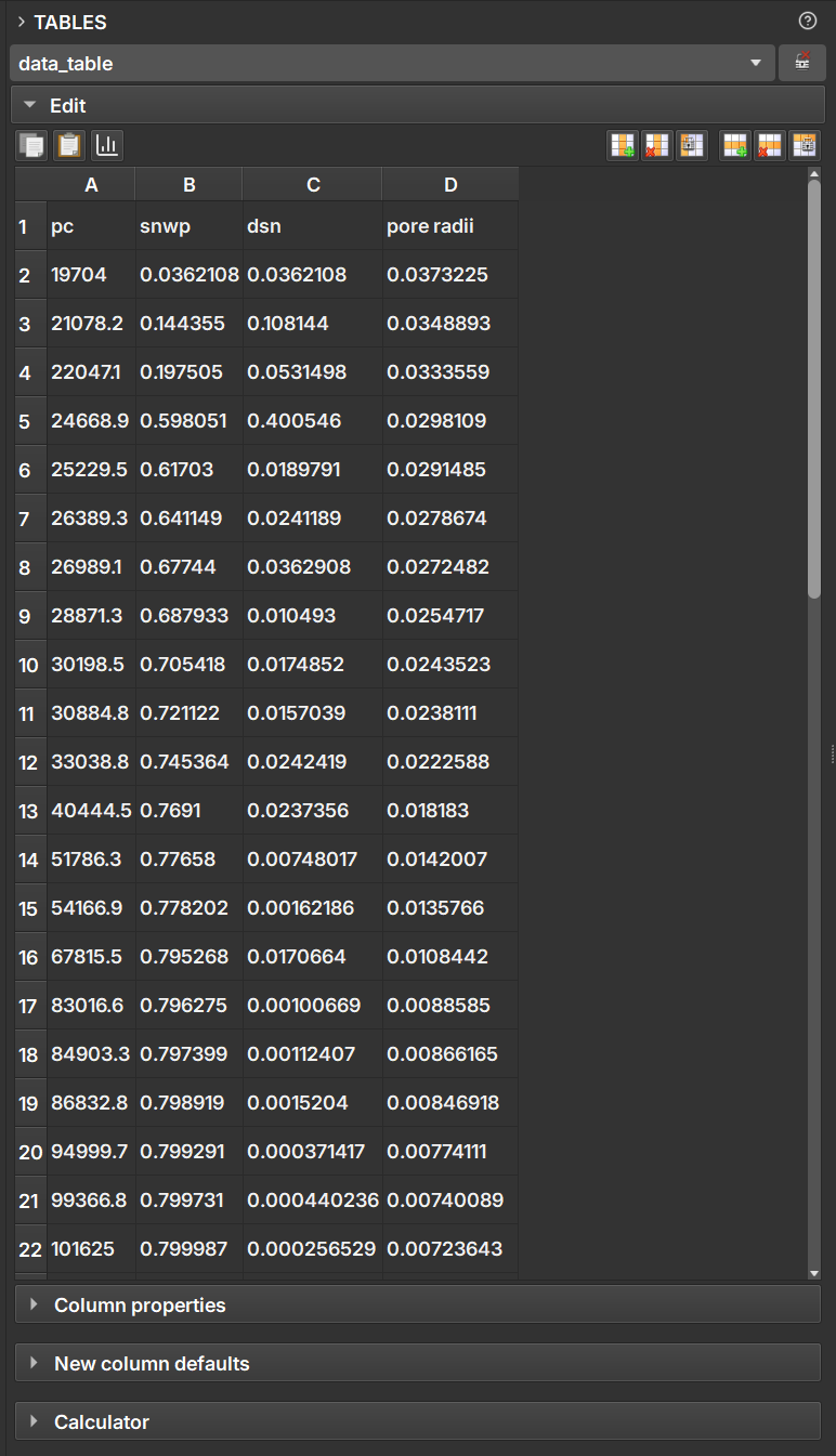
By selecting a table node, the user can edit each of the cells as in a spreadsheet application. From the buttons located above the table, it is also possible to include/remove rows and columns, as well as make copies.
In the Column properties field, you can convert between the data types presented in the table columns.
In the Calculator field, the user can perform simple mathematical operations between the columns to generate new data columns.
Variogram Analysis
The Variogram Analysis module performs an analysis of the spatial correlation and statistical representativeness of data within a given volume.
The variogram is a function that measures the mean squared difference between image values for a given distance between them. Functions that show low values for long distances indicate a greater degree of sample continuity. The module calculates this function for the three image directions (X, Y, and Z) and fits a model to extract parameters such as Range, Sill, and Nugget.

Subvolume analysis is a method for evaluating the Representative Elementary Volume (REV), which corresponds to the smallest volume for which the average of a material's properties becomes constant and representative of the whole. The module determines the REV by analyzing the variation (in the form of standard deviation) of the property's average within subvolumes of increasing sizes. The REV is taken as the low-slope region in the resulting curve.
Inputs
The module uses a unified input panel:
-
Input node: The main volume for analysis. It can be:
vtkMRMLScalarVolumeNode: A grayscale image (e.g., micro-CT image).vtkMRMLLabelMapVolumeNode: A segmented image (label map).vtkMRMLSegmentationNode: A segmentation. If this option is used, the user must select which segments from the list should be analyzed. The analysis will be binary (1 for selected segments, 0 for the rest).
-
Reference: The volume used to define the geometry, spacing (voxel size), and spatial orientation. Generally, it is the same as the input node.
-
Region (SOI): An optional node to define a mask. If an SOI is provided, the entire analysis (Variogram and REV) will be restricted only to voxels within this region.
Parameters
There are two main ways to use the module:
-
Without SOI (FFT Method): If no "Region (SOI)" is provided, the module assumes the user wants to analyze the entire volume. To speed up the calculation, it uses a method based on Fast Fourier Transform (FFT).
-
With SOI (Sampling Method): If a "Region (SOI)" is provided, the module uses a point-pair sampling method within the mask. This method calculates directional variograms (X, Y, Z) and an omnidirectional variogram (r).
The module is divided into two analysis sections. Variogram results calculates the variogram to understand the property's variability in the volume. The parameters of this algorithm are:
Sampling rate: Percentage of points that will be subsampled within the SOI for the calculation. Aims to improve processing time, at the cost of potential accuracy loss.Maximum number of samples: Maximum number of subsampling points that will be used, limiting the sampling defined by theSampling rate. The objective is also to improve processing time, sacrificing accuracy.Number of lags: Defines the number of divisions on the distance axis (X-axis of the variogram), analogous to the number of bins in a histogram.Directional tolerance: Angular tolerance (in degrees) for calculating directional variograms (X, Y, Z). During calculation in a specific direction, the algorithm considers not only perfectly aligned points but also those within this angular tolerance. The objective is to increase statistical robustness, especially in sparse data. For micro-CT data, where point density is high, smaller values (e.g., < 60°) are generally sufficient.Maximum distance: Allows manually defining the maximum distance (in mm) for variogram calculation. If unchecked, it uses a default distance (based on the average).Use nugget: If checked, it takes into account the "Nugget Effect" when fitting the variogram model.
The Representative volume analysis section calculates the standard deviation of the mean as a function of distance. This serves to determine the subvolume size where the property of interest becomes statistically stable. The parameters for this algorithm are:
Number of volume sizes: The number of different edge sizes to be tested (e.g., 10 sizes between minimum and maximum).Maximum number of samples per volume: The number of random subvolumes to be sampled for each size, ensuring statistical robustness.
Results and Outputs
-
Variogram Plots:
- A top bar chart shows the number of point pairs (samples) used at each "lag" (distance).
- The main plot shows the experimental variogram points and the fitted model curve for each direction (X, Y, Z, r).
-
Parameter Table: Below the plot, a table displays the fitted values for Range, Sill, and Nugget for each direction.
-
REV Plot:
- A top bar chart shows the number of samples (subvolumes) used for each size.
- The main plot graphs the Standard Deviation of the Mean (Y-axis) against the Edge Size (X-axis, in mm).
Report Export (HTML)
The module can generate a unified HTML report containing the results of both analyses.
- Export directory: The user specifies the folder where the report will be saved.
- Export report: Upon clicking, the module:
- Extracts metadata from the reference file name (e.g., Well, Plug, Condition, using the convention).
- Captures an image of the current 3D view in Slicer.
- Captures images of the Variogram and REV plots (if they have been calculated).
- Inserts all this information (metadata, images, results tables) into an HTML template (
variogram_report_template.html) and saves it to the export directory.
NetCDF
The NetCDF module provides a set of tools for working with the NetCDF file format (.nc), which is used in GeoSlicer to store multiple volumes, segmentations, and tables in a single self-contained file.
The main advantage of using the NetCDF format is the ability to group related data into a single file. For example, you can save an original image volume and multiple segmentations or analyses (such as porosity tables) together. This keeps all your project data organized and portable, facilitating sharing and archiving.
Additionally, NetCDF is a standard and self-describing data format, widely used in scientific applications. This means that .nc files generated by GeoSlicer can be easily opened and processed by other external tools and libraries, such as xarray and netCDF4 in Python, enabling customized analysis workflows.
Features
The module is divided into three main tabs:
- Import: Allows loading data from a NetCDF (
.nc) or HDF5 (.h5,.hdf5) file into the scene. - Save: Allows saving new images or tables from a project folder back to the original NetCDF file from which they were imported. This operation modifies the existing file.
- Export: Allows exporting one or more items from the scene to a new NetCDF file.
Integration with Other Modules
NetCDF files integrate with other GeoSlicer modules for advanced workflows:
- It is possible to import a NetCDF file using the Micro CT Loader.
- For NetCDF files containing images too large to fit into memory, you can use the Big Image module to view and process them efficiently.
NetCDF Import
The Import tab is used to load data from NetCDF (.nc) or HDF5 (.h5, .hdf5) files into GeoSlicer.
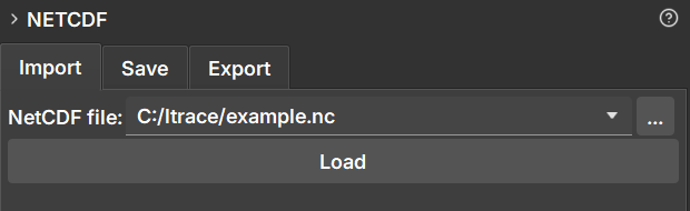
How to Use
- Navigate to the NetCDF module and select the Import tab.
- Click the file selection button next to "NetCDF file:" to open the file explorer.
- Select the
.nc,.h5, or.hdf5file you want to load. - Click the Load button.
Behavior
When loading a file, GeoSlicer creates a new folder in the data hierarchy with the same name as the file. All volumes, segmentations, and tables contained within the NetCDF file are loaded into this folder.
This project folder is linked to the original file. This linking is essential for the Save functionality, which allows updating the original file with new data generated in GeoSlicer.
NetCDF Export
The Export tab allows you to save one or more scene items (volumes, segmentations, tables) into a new NetCDF (.nc) file. It is the ideal tool to create a new dataset from results generated or modified in GeoSlicer.
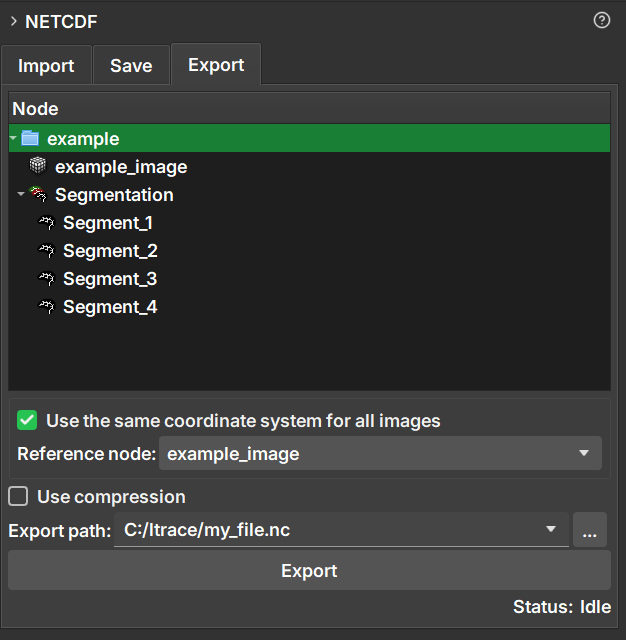
How to Use
- Navigate to the NetCDF module and select the Export tab.
- In the data hierarchy tree displayed in the module, select the items you wish to export. You can select individual items (such as volumes or tables) or entire folders to export all their content.
- Choose the destination path and the name of the new file in the Export path field.
- Configure the export options as needed (detailed below).
- Click the Export button.
Export Options
-
Use the same coordinate system for all images:
- When checked, this option ensures that all exported images are spatially aligned. Images are resampled to fit a common coordinate system, defined by the Reference node.
- This is useful for ensuring alignment, but it can increase the file size if images have very different orientations or spacings, due to the need for padding.
- If unchecked, each image is saved with its own coordinate system, which can result in a smaller file.
-
Reference node:
- Enabled only when the option above is checked.
- Select an image (volume) that will serve as a reference for the coordinate system. All other images will be aligned to this one.
-
Use compression:
- When checked, applies compression to the data, which reduces the final file size.
- Compression can make the process of saving and loading the file slightly slower.
Difference between Export and Save
- Export always creates a new
.ncfile. - Save modifies an existing
.ncfile that was previously imported.
Save Data to an Existing NetCDF File
The Save tab offers a way to update a NetCDF file (.nc) that was previously imported into GeoSlicer. It allows you to add new items (such as volumes, segmentations, or tables) from a project folder back to the original file, modifying it directly.
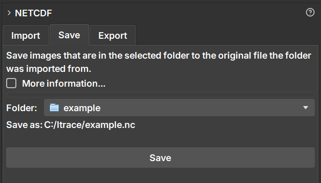
The main motivation for using the Save functionality is to be able to save changes or new data (such as a newly created segmentation) back to the original NetCDF file, preserving all existing attributes, metadata, and coordinate structure. Unlike the "Export" option, which creates an entirely new file, "Save" only appends the new data, ensuring that consistency with the original file is maintained. This is ideal for iterative workflows where you enrich an existing dataset without losing the original context.
How to Use
The Save functionality is designed for a specific workflow:
- First, import a NetCDF file using the Import tab. This will create a project folder in the data hierarchy.
- Work on your project. You can, for example, create a new segmentation for a volume that was in the file or drag a new volume into the project folder.
- Navigate to the NetCDF module and select the Save tab.
- In the Folder field, select the project folder that corresponds to the file you want to update.
- The Save as: field will be automatically populated with the original file path, confirming where the changes will be saved.
- Click the Save button.
Behavior
- The operation modifies the original file. It is recommended to create a backup if you need to preserve the file's previous state.
- Only new items within the project folder that do not yet exist in the
.ncfile will be added. - Items that were already in the file are not overwritten or deleted.
- Newly added images are automatically resampled to align with the coordinate system of the data already existing in the file.
Difference between Save and Export
- Save modifies an existing
.ncfile, preserving its structure and metadata. - Export always creates a new
.ncfile.
Attribute Tools
The Attribute Tools module provides tools for editing image attributes. These attributes can be inspected in the "Attributes" tab in the Explorer module.
Import PCR from file
This tool allows the user to import a PCR file and associate it with a volume. The PCR file contains information which is particularly useful for certain analyses like porosity mapping from saturation.
While PCR information is usually imported alongside the image data (for example, through MicroCT Import or NetCDF Loader), this tool is useful when the PCR data needs to be imported separately or updated.
How to use
- Select a tool: From the "Tool" dropdown menu, select "Import PCR from file".
- Input Volume: Select the volume node that you want to associate the PCR data with.
- PCR File: Click the file browser icon to select the
.pcrfile from your computer. - File Validation: After selecting a file, the module will validate it.
- If the file is a valid PCR file, it will display the minimum and maximum values found in the file.
- If the file is not valid or does not exist, an error message will be displayed.
- Import: Once a valid volume and a valid PCR file are selected, the "Import PCR" button will be enabled. Click it to import the data.
- A success message will appear after the import is complete. The PCR information is now stored within the volume node's metadata. You can verify this by navigating to the Explorer module, selecting the volume, and inspecting the
Attributestab.
Workflows
Tables
In addition to visual reports, Geoslicer allows the export of data tables derived from the analyses performed. These tables are vital for detailed documentation of results, enabling quantitative and comparative analysis, and are easily integrated with other analysis software.
The Tables icon is used to edit tables, as described in the steps below:
- Click on the table icon.
- Browse table data through the interactive window
- In the Calculator section, describe the operation between the columns and the column that will be modified/added
- Click on Calculate to modify the table according to the formula from the previous step.
Graphs
The Graphs icon in GeoSlicer is used for data visualization through various types of graphs, allowing the generation of graphs from data contained in tables. Available graph types include crossplots, rose diagrams, and bar charts. The module's interface allows users to select data tables, choose a graph type, and display multiple datasets on the same graph. The graph interface allows interactive customization, such as adjusting scales and selecting properties for the X, Y, and Z axes.
- Click on the Graph icon.
- Select a table with the data to be used in the plot
- In Plot type, choose the ideal plot type to be rendered with your data
- Click on Plot
- Name your plot and click on Ok
- In the data section, select the column to be plotted
- The options Bins, Show mean and standard deviation and Log mode can be used to improve data visualization
Multiple Image Analysis Module
The Multiple Image Analysis module is an advanced Geoslicer tool, designed to generate custom reports based on different types of image analyses. It supports analyses such as histograms, depth averages, and basic petrophysics. Users can select the desired analysis type through an intuitive interface, load directories containing thin section images, and configure specific options for each analysis type. After processing, the module generates detailed reports that can be viewed and exported for later use. The flexibility in choosing different analysis types allows geologists to gain comprehensive and detailed insights into the properties of the studied rocks.