Image Log Pre-processing
Image Log Crop
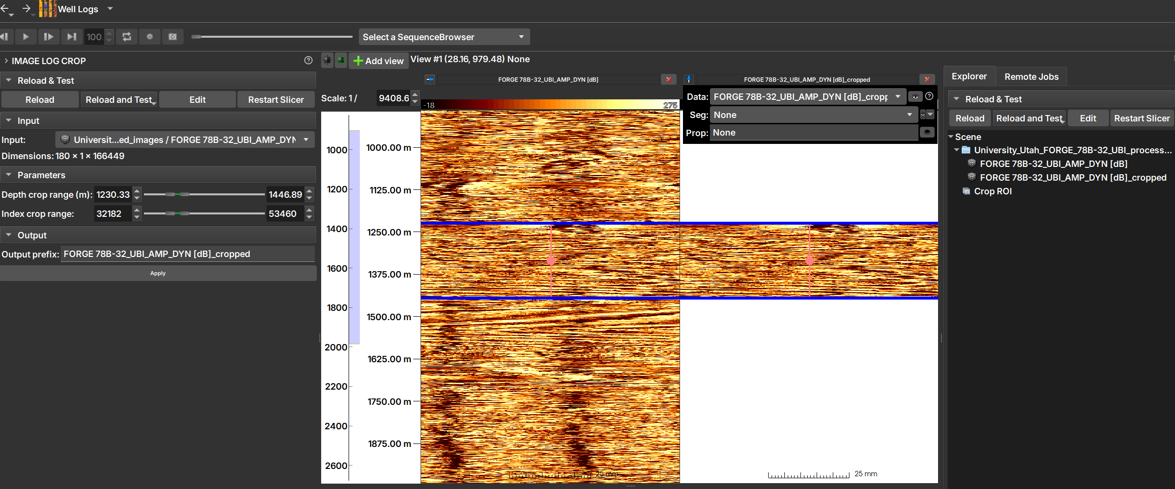
The Image Log Crop Module allows custom cropping of well images, adjusted based on the top and bottom depths of the image.
Panels and their use
 |
|---|
| Figure 1: Manipulation can be done using sliders and numerical values (on the left), or by dragging the crop region with the mouse over the well image (in the center). After clicking "Apply", the cropped image can be opened and viewed, as shown in the image on the right. |
Sliders manipulations (on the left in Image 1) are automatically reflected in the crop region (in the center of the image) and vice-versa.
Main options
-
Input: Choose the image to be cropped.
-
Depth crop range (m): Lower and upper limits of the depth range that will constitute the crop, in meters.
-
Index crop range: The same limits as above, but expressed in indices.
-
By dragging the crop region with the mouse over the well image (in the center)
Azimuth Shift
The Azimuth Correction module applies a rotation to acoustic image profiles (such as UBI) to correct rotational misalignments caused by tool movement in the well.
Acoustic image profiles are unwrapped in 2D, where one dimension is depth and the other is azimuth (0 to 360 degrees). During acquisition, the logging tool can rotate, which distorts the appearance of geological structures.
This module uses an azimuth table to rotate each image line back to its correct orientation, ensuring that geological features are displayed consistently and interpretably.
How to Use
- Image node: Select the image profile you want to correct.
- Azimuth Table: Choose the table that contains the azimuth data. This table should contain a depth column and a column with the azimuth deviation values in degrees.
- Table Column: Select the specific column in the table that contains the azimuth values to be used for correction.
- Invert Direction (Optional): Check this box if you want the rotation to be applied counter-clockwise. By default, the rotation is clockwise.
- Output prefix: Define the name for the corrected image that will be generated.
- Click Apply: Press the button to start the correction process.
Output
The result is a new image in the project with the azimuthal correction applied.
Spiral Filter
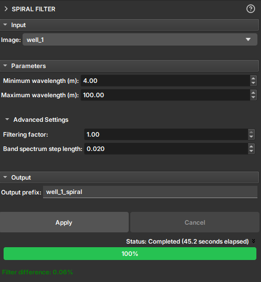
The Spiral Filter module is a tool designed to remove artifacts from image profiles caused by the spiral movement and eccentricity of the logging tool within the well.
During the acquisition of image profiles, the rotational movement of the tool (spiraling) and its misalignment relative to the center of the well (eccentricity) can introduce periodic noise into the images. This noise appears as a pattern of bands or spirals superimposed on the geological data, which can make the interpretation of true features difficult.
This filter operates in the frequency domain to selectively remove signal components associated with these artifacts, resulting in a cleaner and easier-to-interpret image.
How It Works
The filter is based on applying a band-stop filter to the 2D Fourier transform of the image. The frequency band to be rejected is defined by the vertical wavelengths (in meters) that correspond to the visible spiral pattern in the image. The user can measure these wavelengths directly on the image using the ruler tool to configure the filter parameters.
How to Use
- Image: Select the image profile you want to filter.
- Parameters:
- Minimum wavelength (m): Define the minimum vertical wavelength of the spiral artifact. This value corresponds to the smallest vertical repetition distance of the pattern.
- Maximum wavelength (m): Define the maximum vertical wavelength of the artifact.
- Advanced Settings (Optional):
- Filtering factor: Control the filter intensity. A value of
0applies no filtering, while1applies maximum filtering. - Band spectrum step length: Adjusts the smoothness of the filter's frequency band transition. Larger values result in a smoother transition.
- Filtering factor: Control the filter intensity. A value of
- Output prefix: Define the name for the new filtered image volume.
- Click Apply: Press the button to start the filtering process.
Output
The result is a new image volume in the scene with the filter applied. After execution, the Filter difference field displays the percentage of the image that was changed by the filter, providing a quantitative measure of the filtering impact.
Image Log Inpaint
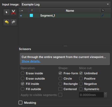
The Image Log Inpaint Module integrated into GeoSlicer is an inpainting tool that allows interactive inpainting of missing or damaged areas in well images, with dynamic adjustments during the process.
Panels and their usage
 |
|---|
| Figure 1: Presentation of the Image Log Crop module. |
Main options
-
Input image: Choose the image to be inpainted. When an image is chosen, two views will be automatically added to facilitate usability.
-
Clone Volume: Creates a new image to be used in the module, keeping the original image unchanged.
-
Rename Volume: Renames the chosen image.
-
Tesoura/Scissors: Tool that performs the inpainting: first, select the tool and then draw on the image the area where the inpainting should be performed. The tool options in the bottom menu are disabled in this module.
-
Arrows: Allow to undo or redo an inpainting modification.
CLAHE Tool
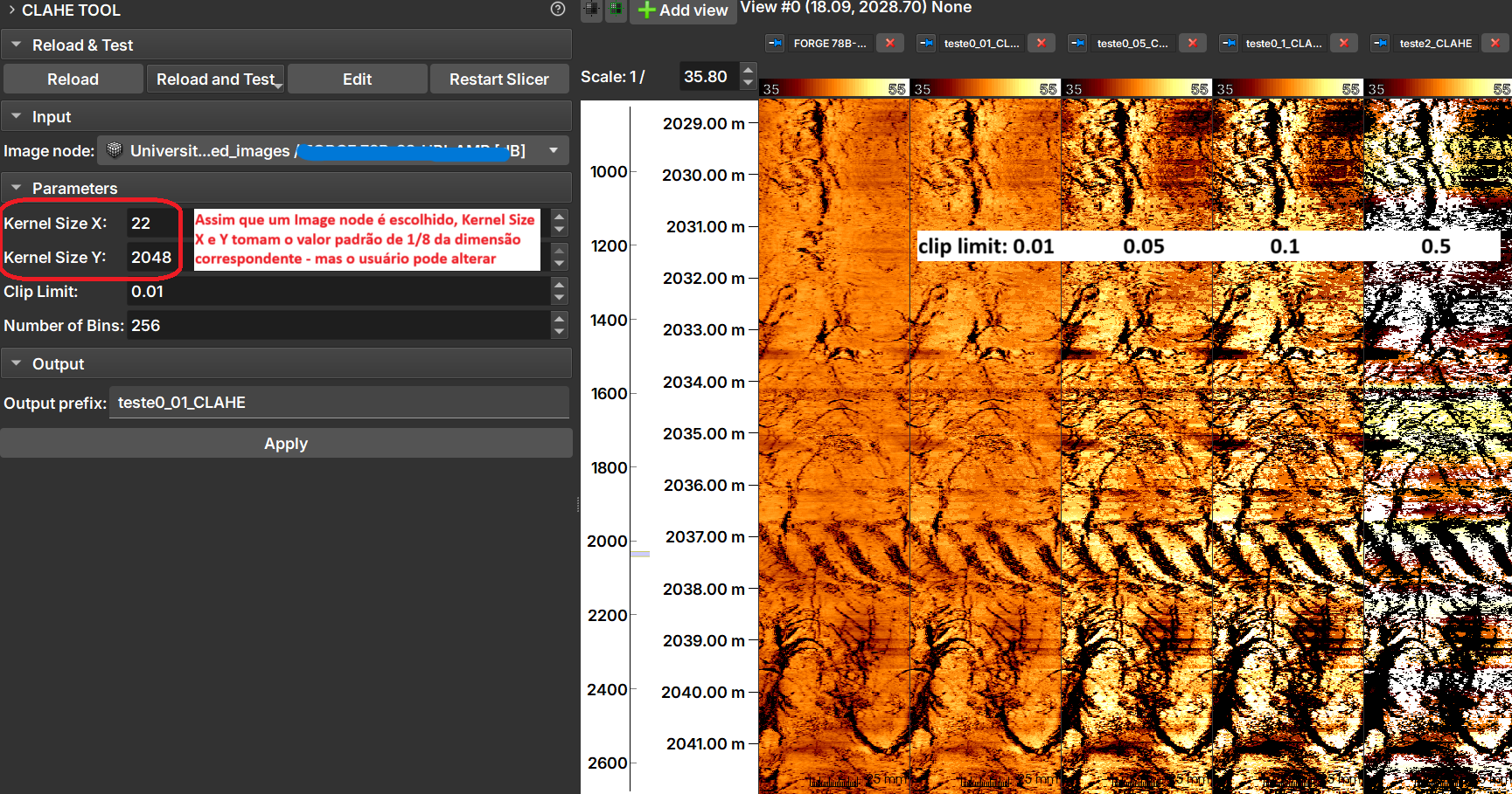
The CLAHE Tool Module applies Contrast Limit Adaptive Histogram Equalization (CLAHE), "an algorithm for local contrast enhancement, which uses histograms computed over different regions of an image. Thus, local details can be enhanced even in regions lighter or darker than most of the image" - documentation of the equalize_adapthist function from scikit-image on 06/25/2025.
Panels and their usage
 |
|---|
| Figure 1: CLAHE Tool module presentation. |
The image shows the result of applying CLAHE with different clip limit values.
Inputs
- Image Node: Image Log volume to be processed.
Parameters
- Kernel Size: Defines the shape of the contextual regions used in the algorithm. By default, kernel_size is 1/8 of the image height by 1/8 of the width.
- Clip Limit: Normalized between zero 0 and 1. High values result in higher contrast.
- Number of Bins: Number of bins for the histograms ('data range').
Outputs
- Output prefix: Processed image, with float64 type.